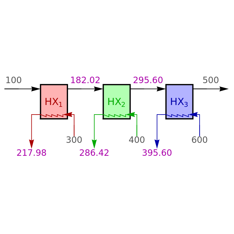
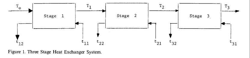
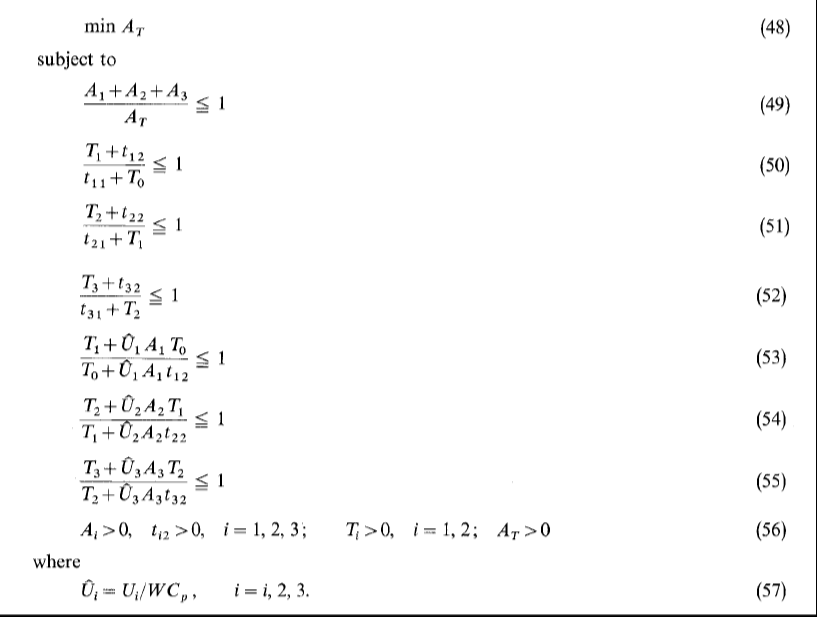
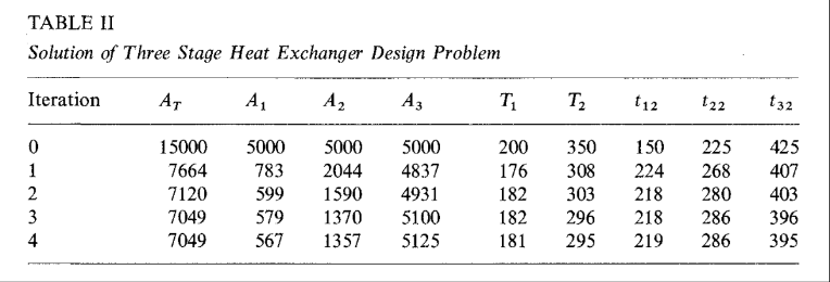
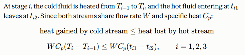
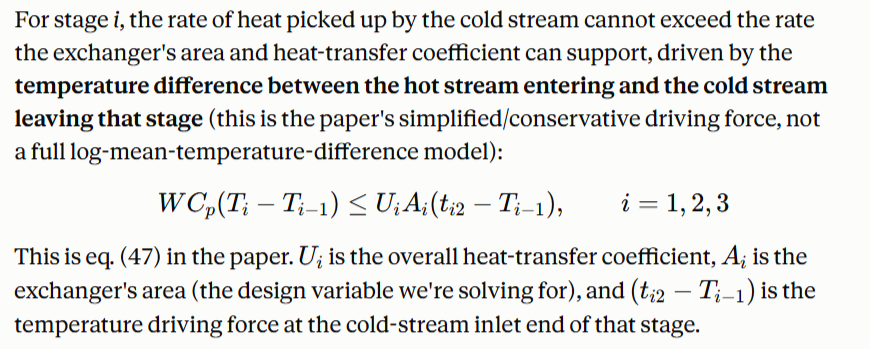
Consider a three-stage heat exchanger optimal design problem[1, 2]. A cold fluid is heated from 100 °F to 500 °F by passing through three heat exchangers in series (labeled , , and in the diagram). At each stage, the cold stream is heated by a hot fluid whose inlet temperature is fixed at 300°F, 400°F, and 600°F for stages 1, 2, and 3, respectively. The overall heat transfer coefficients (expressed in Btu/hr ºF) of these exchangers are equal to =120, =80, and =40. Assume that the hot and cold fluids have the same flow rate and specific heat , and that Btu/hr ºF.We seek the optimal design, which minimizes the overall area or =++, where is the area of the heat exchanger. Rather than implementing the paper's iterative complementary-geometric-programming algorithm, this notebook solves the resulting nonlinear program directly with FindMinimum. It computes all the unknown temperatures (expressed in °F and shown in magenta in the diagram) and, in the summary table below the diagram, the values of the areas of the three heat exchangers that minimize .A detailed mathematical formulation of the problem (objective function and inequality constraints) is given below [1, 2].The minimum total area found below, about 7049.25 sq. ft., matches the value that [1] reports after four iterations of its original iterative posynomial-approximation algorithm (Table II).[1] M. Avriel and A. C. Williams, "An Extension of Geometric Programming with Applications in Engineering Optimization," Journal of Engineering Mathetmatics, 5(2), 1971 pp. 187–194. doi10.1007/BF01535411.[2] N. Andrei, Nonlinear Optimization Applications Using the GAMS Technology, New York: Springer, 2013.
HX
1
HX
2
HX
3
2
ft
U
1
U
2
U
3
W
C
P
W×=
C
P
5
10
A
total
A
1
A
2
A
3
A
i
th
i
A
total
In[]:=
Print["temperature of hot fluid entering the heat exchangers (ºF) "];t11=300;t21=400;t31=600;Print[t11," ",t21," ",t31];
temperature of hot fluid entering the heat exchangers (ºF)
300 400 600
In[]:=
U1h=U1/(WCp);U2h=U2/(WCp);U3h=U3/(WCp);W=10^5/Cp;T0=100;T3=500;U1=120;U2=80;U3=40;
In[]:=
sol=FindMinimum[{AT,(A1+A2+A3)/AT≤1,(T1+t12)/(t11+T0)≤1,(T2+t22)/(t21+T1)≤1,(T3+t32)/(t31+T2)≤1,(T1+U1hA1T0)/(T0+U1hA1t12)≤1,(T2+U2hA2T1)/(T1+U2hA2t22)≤1,(T3+U3hA3T2)/(T2+U3hA3t32)≤1,AT>0,A1>0,A2>0,A3>0,t12>0,t22>0,t32>0,T1>0,T2>0},{AT,15000},{A1,5000},{A2,5000},{A3,5000},{T1,200},{T2,350},{t12,150},{t22,225},{t32,425}]
Out[]=
{7049.25,{AT7049.25,A1579.307,A21359.97,A35109.97,T1182.018,T2295.601,t12217.982,t22286.416,t32395.601}}
All six inequality constraints are active at the optimum: both the three heat-balance constraints and the three heat-transfer constraints
are binding simultaneously.None of them is slack.
This isn't a coincidence—it's exactly what Avriel& Williams show. For a well-posed geometric (or complementary geometric) program, the optimum lies where all—or,more precisely,enough of—the constraints are tight, and this connects directly to the "degree of difficulty" discussion in the paper: the paper counts this problem as having 15−9 = 6 degrees of difficulty, matching that there are 6 active constraints pinning down the 9 primal variables (AT, A₁, A₂, A₃, T₁, T₂, t₁₂, t₂₂, t₃₂) relative to the objective.
In[]:=
{(A1+A2+A3)/AT,(T1+t12)/(t11+T0),(T2+t22)/(t21+T1),(T3+t32)/(t31+T2),(T1+U1hA1T0)/(T0+U1hA1t12),(T2+U2hA2T1)/(T1+U2hA2t22),(T3+U3hA3T2)/(T2+U3hA3t32)}/.sol[[2]]
Out[]=
{1.,1.,1.,1.,1.,1.,1.}
In[]:=
p1=Show[Graphics[{EdgeForm[Thick],Opacity[0.3],Red,Rectangle[{1,1},{4,5}],Opacity[0.3],Green,Rectangle[{8,1},{11,5}],Opacity[0.3],Blue,Rectangle[{15,1},{18,5}],Black,Opacity[1],Arrow[{{-3,4.5},{1,4.5}}],Arrow[{{4,4.5},{8,4.5}}],Arrow[{{11,4.5},{15,4.5}}],Arrow[{{18,4.5},{22,4.5}}],Darker@Red,Arrow[{{4.75,-1},{4.75,1.5},{3.5,1.5}}],Arrow[{{1,1.5},{0.0,1.5},{0.0,-2.5}}],Table[Line[{{1+(i-1)(3.5-1)/4,1.5},{1+i(3.5-1)/4,1.25}}],{i,1,4}],Table[Line[{{1+(i-1)(3.5-1)/4,1.5},{1+(i-1)(3.5-1)/4,1.25}}],{i,2,5}],Darker@Green,Arrow[{{11.75,-1},{11.75,1.5},{10.5,1.5}}],Arrow[{{8,1.5},{7.0,1.5},{7.0,-2.5}}],Table[Line[{{8+(i-1)(10.5-8)/4,1.5},{8+i(10.5-8)/4,1.25}}],{i,1,4}],Table[Line[{{8+(i-1)(10.5-8)/4,1.5},{8+(i-1)(10.5-8)/4,1.25}}],{i,2,5}],Darker@Blue,Arrow[{{18.75,-1},{18.75,1.5},{17.5,1.5}}],Arrow[{{15,1.5},{14.0,1.5},{14.0,-2.5}}],Table[Line[{{15+(i-1)(17.5-15)/4,1.5},{15+i(17.5-15)/4,1.25}}],{i,1,4}],Table[Line[{{15+(i-1)(17.5-15)/4,1.5},{15+(i-1)(17.5-15)/4,1.25}}],{i,2,5}],Style[Text["",{2.5,3.0},{0,0}],Darker@Red,16],Style[Text["",{9.5,3.0},{0,0}],Darker@Green,16],Style[Text["",{16.5,3.0},{0,0}],Darker@Blue,16],Style[Text[NumberForm[T0,{4,2}],{-2.0,5.5},{0,0}],Darker@Gray,14],Style[Text[NumberForm[T3,{4,2}],{20.0,5.5},{0,0}],Darker@Gray,14],Style[Text[NumberForm[T1/.sol[[2]],{5,2}],{6.0,5.5},{0,0}],Darker@Magenta,14],Style[Text[NumberForm[T2/.sol[[2]],{5,2}],{13.0,5.5},{0,0}],Darker@Magenta,14],Style[Text[NumberForm[t11,{4,1}],{4.75,-1.5},{0,0}],Darker@Gray,14],Style[Text[NumberForm[t21,{4,1}],{11.75,-1.5},{0,0}],Darker@Gray,14],Style[Text[NumberForm[t31,{4,1}],{18.75,-1.5},{0,0}],Darker@Gray,14],Style[Text[NumberForm[t12/.sol[[2]],{5,2}],{0.0,-3.0},{0,0}],Darker@Magenta,14],Style[Text[NumberForm[t22/.sol[[2]],{5,2}],{7.0,-3.0},{0,0}],Darker@Magenta,14],Style[Text[NumberForm[t32/.sol[[2]],{5,2}],{14.0,-3.0},{0,0}],Darker@Magenta,14]}],AspectRatio0.35,ImageSize380{1,1}]
HX
1
HX
2
HX
3
Out[]=