The latest versions of Mathematica allows as to calculate convection even with . Data below has been computed with the code in this notebook. It takes a time to finish computation at t=1. Code has been developed by Lion Sahara and debugged here in my answer. In the picture above shown velocity field animated with step dt=0.01. We see the turbulent like convection
Ra=
7
10
In[]:=
Needs["NDSolve`FEM`"];
In[]:=
ResourceFunction["FEMAddOnsInstall"][]
Out[]=
PacletObject

In[]:=
Needs["FEMAddOns`"]
In[]:=
ClearAll[length,height,offsetx1,offsetx2,offsety];sizes={length->21/10,height->15/10,offsetx1->1/10,offsetx2->1/10,offsety1->1/10,offsety2->2/10};
Geometry
Geometry
In[]:=
Ω1=Rectangle[{0,0},{length,height}]/.sizes;Ω2=Rectangle[{0,0}+{0.2,1.5-0.049},{0.69,0.049}+{0.2,1.5-0.049}];ΩD1=RegionDifference[Ω1,Ω2]
Out[]=
Polygon

In[]:=
Ω3=Rectangle[{0,0}+{1.2,1.5-0.049},{0.69,0.049}+{1.2,1.5-0.049}];ΩD2=RegionDifference[ΩD1,Ω3]
Out[]=
Polygon

In[]:=
{Region[ΩD1,AspectRatio->Automatic],Region[ΩD2,AspectRatio->Automatic]}
Out[]=
,


Mesh
Mesh
In[]:=
Ω=DiscretizeRegion[ΩD2,MaxCellMeasure0.001,AccuracyGoal5,PrecisionGoal5]
Out[]=
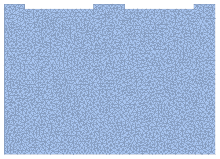
In[]:=
meshes=ToBoundaryMesh/@{Ω1,Ω2,Ω3};
In[]:=
bmesh=FEMUtils`BoundaryElementMeshJoin@@meshes;
In[]:=
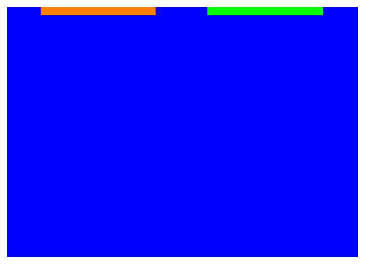
boxCoordinate={1.05,0.8};PCMCoordinate1={0.5,1.46};PCMCoordinate2={1.5,1.46};markerColors={Blue,Orange,Green};markerCoordinate={{boxCoordinate},{PCMCoordinate1},{PCMCoordinate2}};
In[]:=
markerspec=MapIndexed[{First@#1,First@#2}&,markerCoordinate]
Out[]=
{{{1.05,0.8},1},{{0.5,1.46},2},{{1.5,1.46},3}}
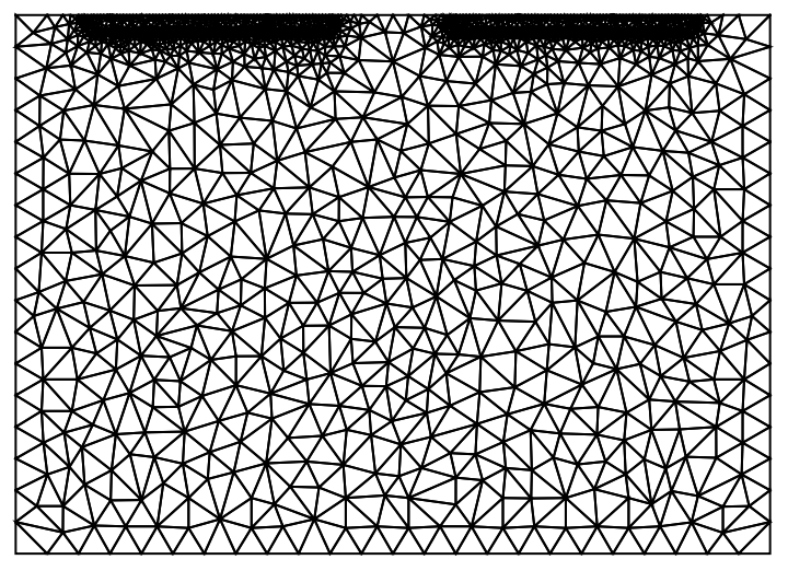
mesh=ToElementMesh[bmesh,"RegionMarker"->markerspec,"MaxCellMeasure"->5*10^-3];
In[]:=
mesh["Wireframe"[]]
Out[]=
In[]:=
mesh["Wireframe"["MeshElementStyle"->Map[Directive[FaceForm[#],EdgeForm[]]&,markerColors]]]
Out[]=
In[]:=
Show[{bmesh["Wireframe"],Graphics[MapThread[{PointSize[0.02],#1,Point/@#2}&,{markerColors,markerCoordinate}]]}]
Out[]=
Material Properties
Material Properties
In[]:=
region=<|"air"->1,"pcm"->2|>
Out[]=
air1,pcm2
In[]:=
vars={T[t,x,y],t,{x,y}};HeatTransferPDEComponent[vars,<|"MassDensity"->ρ,"SpecificHeatCapacity"->Cp,"ThermalConductivity"->k|>]
Out[]=
∇
{x,y}
∇
{x,y}
(1,0,0)
T
In[]:=
airpara=->QuantityMagnitude[ThermodynamicData["Air","Density"]], ->QuantityMagnitude[ThermodynamicData["Air","IsobaricHeatCapacity"]], ->QuantityMagnitude[ThermodynamicData["Air","ThermalConductivity"]]
ρ
air
Cp
air
k
air
Out[]=
{1.20458,1006.14,0.0258738}
ρ
air
Cp
air
k
air
In[]:=
HS30Npara=->2.1,->2.7, ->2.34,->0.6, ->1430,latent->200, tpmin->-34,tpmax->-26;
Cp
pcmS
Cp
pcmL
k
pcmS
k
pcmL
ρ
pcmS
In[]:=
PUFpara={ρ->50,cp->1500,k->0.025};
In[]:=
pars=<||>;pars["MassDensity"]=If[ElementMarker==region["air"],,];pars["SpecificHeatCapacity"]=If[ElementMarker==region["air"],,];pars["ThermalConductivity"]=If[ElementMarker==region["air"],,*IdentityMatrix[2]];
ρ
air
ρ
pcmS
k
air
k
pcmS
k
air
k
pcmS
In[]:=
op=HeatTransferPDEComponent[vars,pars]
Out[]=
∇
{x,y}
k
air
k
pcmS
∇
{x,y}
k
air
k
pcmS
ρ
air
ρ
pcmS
(1,0,0)
T
Initial and Boundary Condition
Initial and Boundary Condition
CITE THIS NOTEBOOK
CITE THIS NOTEBOOK
Convection of air with higher Rayleigh number
by Alexander Trounev
Wolfram Community, STAFF PICKS, February 2, 2024
https://community.wolfram.com/groups/-/m/t/3115061
by Alexander Trounev
Wolfram Community, STAFF PICKS, February 2, 2024
https://community.wolfram.com/groups/-/m/t/3115061