Poiseuille Flow in a Rectangular Channel
Authors: Housam Binous and Ahmed Bellagi
Poiseuille Flow in a Rectangular Channel
Authors: Housam Binous and Ahmed Bellagi
Authors: Housam Binous and Ahmed Bellagi
We solve the Poiseuille flow problem in a rectangular channel using the finite differences approach (for details see Ref. 1) . The result obtained using this numerical technique is in agreement with the one given by the analytical solution (given in Ref. 2), which was derived using separation of variables . We also compare our results with their counterpart obtained using NDSolve.Governing equation is a Partial Differential Equation (PDE) called the Poisson equation: In addition, we assume the no-slip boundary conditions are valid.Without loss of generality, we assume f = 5 and H = L = 1 .For a solution using Chebyshev orthogonal collocation see Ref. 3.References :1- Kenneth J. Beers, Numerical Methods for Chemical Engineering, Applications in Matlab, Cambridge University Press, 2007, pp. 260-264.2- T. D. Bennett, Transport by advection and diffusion, Wiley, NewYork, 2013, pp. 111-115.3- H. Binous, S. Kaddeche and A. Bellagi, Solving Two-Dimensional Chemical Engineering Problems using the Chebyshev Orthogonal Collocation Technique, Computer Applications in Engineering Education, 24(1), pp. 144-155, 2016.
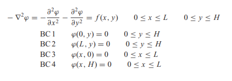
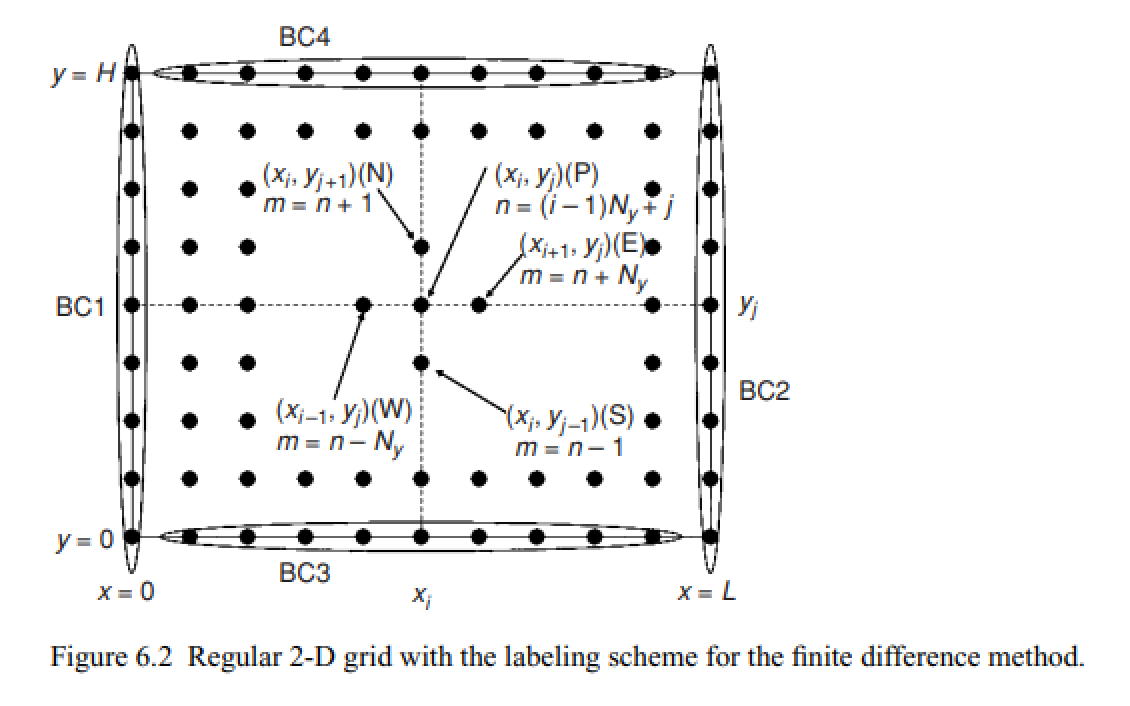
Poiseuille Flow in a rectangular channel using finite differences.Discretization of the PDE yields a set of linear equations for each node (xi, yj) :Finally, we take : Δx=1/29. Hence, we use for the finite diffrences method 30 equally-spaced nodes.

In[]:=
Np=30;
In[]:=
Np^2
Out[]=
900
In[]:=
t=Table[a[i,j],{i,1,900},{j,1,900}];
In[]:=
Δx=1/29.
Out[]=
0.0344828
In[]:=
For[i=1,i<901,{For[j=1,j<901,{a[i,j]=0,j++}],i++}]
In[]:=
For[k=31,k<871,{If[Mod[k,30]≠1&&Mod[k,30]≠0,a[k,k]=4/Δx^2],k++}]
In[]:=
For[k=31,k<871,{If[Mod[k,30]0||Mod[k,30]1,a[k,k]=1],k++}]
In[]:=
For[k=1,k<31,{a[k,k]=1,k++}]
In[]:=
For[k=871,k<901,{a[k,k]=1,k++}]
In[]:=
For[k=30,k<871,{If[Mod[k,30]≠1&&Mod[k,30]≠0,{a[k,k-1]=-1/Δx^2,a[k,k+1]=-1/Δx^2}],k++}]
In[]:=
For[k=30,k<871,{If[Mod[k,30]≠1&&Mod[k,30]≠0,{a[k,k-30]=-1./Δx^2,a[k,k+30]=-1/Δx^2}],k++}]
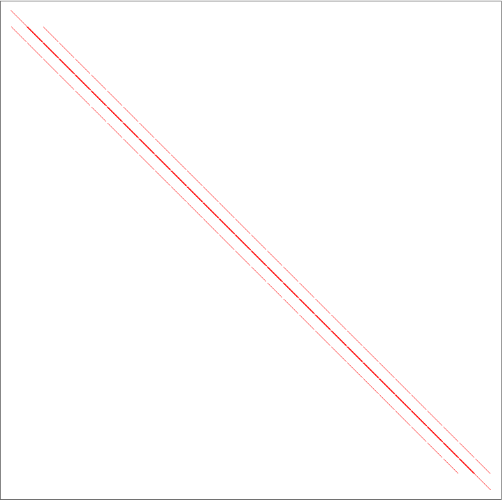
Since each discretized equation involves only 5 nodes, the matrix labeled t is a banded matrix
In[]:=
ArrayPlot[t,ColorRules{0White,0.White,_Red}]
Out[]=
In[]:=
c=Table[b[i,j],{i,1,30},{j,1,30}];
In[]:=
For[i=1,i<31,{For[j=1,j<31,{b[i,j]=5,j++}],i++}]
In[]:=
For[k=1,k<31,{b[1,k]=0,k++}]
In[]:=
For[k=1,k<31,{b[30,k]=0,k++}]
In[]:=
For[i=1,i<31,{For[j=1,j<31,{If[Mod[j,30]1||Mod[j,30]0,b[i,j]=0],j++}],i++}]
In[]:=
c
Out[]=
{{0,0,0,0,0,0,0,0,0,0,0,0,0,0,0,0,0,0,0,0,0,0,0,0,0,0,0,0,0,0},{0,5,5,5,5,5,5,5,5,5,5,5,5,5,5,5,5,5,5,5,5,5,5,5,5,5,5,5,5,0},{0,5,5,5,5,5,5,5,5,5,5,5,5,5,5,5,5,5,5,5,5,5,5,5,5,5,5,5,5,0},{0,5,5,5,5,5,5,5,5,5,5,5,5,5,5,5,5,5,5,5,5,5,5,5,5,5,5,5,5,0},{0,5,5,5,5,5,5,5,5,5,5,5,5,5,5,5,5,5,5,5,5,5,5,5,5,5,5,5,5,0},{0,5,5,5,5,5,5,5,5,5,5,5,5,5,5,5,5,5,5,5,5,5,5,5,5,5,5,5,5,0},{0,5,5,5,5,5,5,5,5,5,5,5,5,5,5,5,5,5,5,5,5,5,5,5,5,5,5,5,5,0},{0,5,5,5,5,5,5,5,5,5,5,5,5,5,5,5,5,5,5,5,5,5,5,5,5,5,5,5,5,0},{0,5,5,5,5,5,5,5,5,5,5,5,5,5,5,5,5,5,5,5,5,5,5,5,5,5,5,5,5,0},{0,5,5,5,5,5,5,5,5,5,5,5,5,5,5,5,5,5,5,5,5,5,5,5,5,5,5,5,5,0},{0,5,5,5,5,5,5,5,5,5,5,5,5,5,5,5,5,5,5,5,5,5,5,5,5,5,5,5,5,0},{0,5,5,5,5,5,5,5,5,5,5,5,5,5,5,5,5,5,5,5,5,5,5,5,5,5,5,5,5,0},{0,5,5,5,5,5,5,5,5,5,5,5,5,5,5,5,5,5,5,5,5,5,5,5,5,5,5,5,5,0},{0,5,5,5,5,5,5,5,5,5,5,5,5,5,5,5,5,5,5,5,5,5,5,5,5,5,5,5,5,0},{0,5,5,5,5,5,5,5,5,5,5,5,5,5,5,5,5,5,5,5,5,5,5,5,5,5,5,5,5,0},{0,5,5,5,5,5,5,5,5,5,5,5,5,5,5,5,5,5,5,5,5,5,5,5,5,5,5,5,5,0},{0,5,5,5,5,5,5,5,5,5,5,5,5,5,5,5,5,5,5,5,5,5,5,5,5,5,5,5,5,0},{0,5,5,5,5,5,5,5,5,5,5,5,5,5,5,5,5,5,5,5,5,5,5,5,5,5,5,5,5,0},{0,5,5,5,5,5,5,5,5,5,5,5,5,5,5,5,5,5,5,5,5,5,5,5,5,5,5,5,5,0},{0,5,5,5,5,5,5,5,5,5,5,5,5,5,5,5,5,5,5,5,5,5,5,5,5,5,5,5,5,0},{0,5,5,5,5,5,5,5,5,5,5,5,5,5,5,5,5,5,5,5,5,5,5,5,5,5,5,5,5,0},{0,5,5,5,5,5,5,5,5,5,5,5,5,5,5,5,5,5,5,5,5,5,5,5,5,5,5,5,5,0},{0,5,5,5,5,5,5,5,5,5,5,5,5,5,5,5,5,5,5,5,5,5,5,5,5,5,5,5,5,0},{0,5,5,5,5,5,5,5,5,5,5,5,5,5,5,5,5,5,5,5,5,5,5,5,5,5,5,5,5,0},{0,5,5,5,5,5,5,5,5,5,5,5,5,5,5,5,5,5,5,5,5,5,5,5,5,5,5,5,5,0},{0,5,5,5,5,5,5,5,5,5,5,5,5,5,5,5,5,5,5,5,5,5,5,5,5,5,5,5,5,0},{0,5,5,5,5,5,5,5,5,5,5,5,5,5,5,5,5,5,5,5,5,5,5,5,5,5,5,5,5,0},{0,5,5,5,5,5,5,5,5,5,5,5,5,5,5,5,5,5,5,5,5,5,5,5,5,5,5,5,5,0},{0,5,5,5,5,5,5,5,5,5,5,5,5,5,5,5,5,5,5,5,5,5,5,5,5,5,5,5,5,0},{0,0,0,0,0,0,0,0,0,0,0,0,0,0,0,0,0,0,0,0,0,0,0,0,0,0,0,0,0,0}}
Here, solution of the system of linear algebraic equations is obtained using matrix inversion. Applying LU factorisation to matrix t is not interesting since it results in the band being filled in by many non-zero elements.
Putting the solution in proper format for ListPlot3D, ListContourPlot and ListDensityPlot commands.
Poiseuille Flow in a rectangular channel using NDSolve
Comparison of the three methods (@ x= 4*Δx= 0.137931) indicates very good agreement