The two faces of urban scaling. Left: a town densifies into a "social reactor" — as people pack closer the interaction web thickens and each resident's output climbs (×1.0 ×1.55). Right: the same growth, two ways — socioeconomic output per person rises (β > 1) while the infrastructure each person needs falls (β < 1).
Abstract
Abstract
When a city doubles in population, its road network does not double — in our UK data its major-road length grows by only about 80%. Its economic output, by contrast, more than doubles: gross value added and business counts both grow by about 120%. These regularities, first documented systematically by Luís Bettencourt and collaborators at the Santa Fe Institute, recur across many countries and decades — although, as we discuss, the precise exponents depend on how a “city” is delineated. They suggest that cities are not merely large villages but are governed by scaling laws rooted in the geometry of social networks and physical infrastructure.
This notebook does four things. First, it derives the theoretical framework from first principles: why infrastructure should scale sublinearly (β ≈ 0.85), why individual needs should scale linearly (β ≈ 1.0), and why socioeconomic outputs should scale superlinearly (β ≈ 1.15). Second, it fits these power laws to real, openly-licensed data on 46 UK cities (population, GVA, business counts, employment and road length from the ONS and the Department for Transport, all under the Open Government Licence). Third, it performs residual analysis to identify which cities over- and under-perform for their size. Fourth, it compares the UK results with international findings and discusses policy implications. Every figure is produced live by a one-line call to the companion package, so the whole analysis is reproducible from the notebook itself.
Audience: the prose is written for two overlapping audiences. Each section opens with an intuitive explanation that requires no background, then deepens into a quantitative treatment with equations, regression code, and confidence intervals. Urban scientists will recognise the canonical references; general readers should be able to follow the scaling narrative and the policy discussion.
1. The puzzle: why cities are not just big villages
1. The puzzle: why cities are not just big villages
Consider two British cities from our dataset: Manchester (population about 590,000) and London (about 9.1 million, aggregated across its 33 boroughs). London is roughly 15 times larger. If cities were just scaled-up versions of each other — big villages — we would expect every measurable quantity to be about 15 times larger in London. But that is not what the data show.
London's economic output (GVA) is about 22 times Manchester's, and its business count about 23 times — more than 15. But its major-road network is only about 13 times longer — less than 15. These ratios (22, 23, 13 against the expected 15) are not random noise: as the regressions in §5 show, they reflect a systematic pattern that recurs across the UK urban system, and similar patterns appear in many countries — though the exact exponents depend on how city boundaries are drawn.
The pattern is this: infrastructure (roads, pipes, cables) grows slower than population. Individual needs (housing, water consumption) grow in proportion to population. And socioeconomic outputs (economic activity, innovation, crime, wages) grow faster than population. The first represents economies of scale: you can serve more people with proportionally less infrastructure. The last represents increasing returns: putting more people together in a dense urban environment produces disproportionately more economic and social activity. Cities are, in Bettencourt's memorable phrase, social reactors — the human interactions that drive innovation and wealth (and also crime and disease) accelerate superlinearly with size.
The mathematical framework for this is the urban scaling law:
Y=·
Y
0
β
N
where Y is a city-level metric, N is population, is a normalisation constant, and β is the scaling exponent. The theoretical predictions — and the empirical results from dozens of studies — give:
Y
0
• β ≈ 0.85 for infrastructure (sublinear: economies of scale)
• β ≈ 1.0 for individual needs (linear)
• β ≈ 1.15 for socioeconomic outputs (superlinear: increasing returns)
These are not arbitrary numbers. As we will show in §3, they follow from the geometry of fractal infrastructure networks and the density of social interactions in cities. The round figures 0.85 and 1.15 are the values commonly quoted in the literature; the clean geometric derivation in §3 actually predicts 5/6 ≈ 0.83 and 7/6 ≈ 1.17, symmetric about 1 with both deviations equal to exactly 1/6 ≈ 0.17. We use the rounded 0.85 / 1.15 as a reference throughout, but keep the exact 5/6, 7/6 in mind when comparing with our fitted exponents.
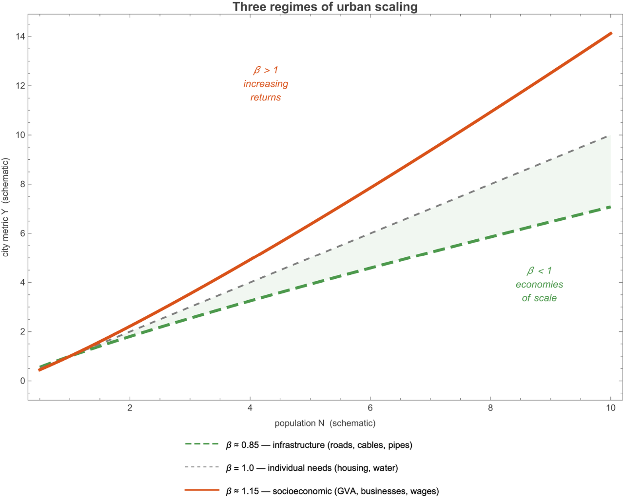
Figure 1.1 The three regimes of urban scaling. Infrastructure (green, dashed) grows sublinearly; individual needs (grey, dotted) grow linearly; socioeconomic outputs (orange, solid) grow superlinearly. The exponents are approximately symmetric around β = 1.
2. Urban scaling laws: the empirical facts
2. Urban scaling laws: the empirical facts
A brief history. The idea that cities exhibit regular quantitative relationships between size and function goes back at least to Zipf (1949), who noted the power-law distribution of city sizes. The modern scaling-law programme was launched by Bettencourt, Lobo, Helbing, Kühnert, and West (2007), who systematically fitted Y = Y₀ to data on hundreds of US and European cities across dozens of metrics. Their key finding: the exponents cluster into three groups, corresponding to the three categories above, with remarkable consistency.
β
N
Subsequent work by Bettencourt (2013) provided a theoretical derivation of these exponents from first principles — a mean-field model of a city as a social network embedded in a fractal infrastructure geometry. West (2017) synthesised the scaling programme into a popular-science book. Batty (2013) placed the results in the broader context of urban science and complexity theory.
The scaling approach is log-linear. Taking logarithms of both sides of the power law:
lnY=ln+βlnN
Y
0
This is an ordinary linear regression in log-log space. The slope is β; the intercept is ln Y₀. The R² of this regression is typically 0.9–0.99 for well-defined metrics, indicating that population alone explains the vast majority of variation in city-level quantities.
Why power laws? A power law Y ∝ is the unique functional form that is scale-invariant: it has no characteristic size. If you double the population, the metric changes by a factor — regardless of whether you started with a town of 50,000 or a metropolis of 5,000,000. This is a strong constraint on the underlying mechanisms: whatever drives the relationship must itself be scale-free.
β
N
β
2
3. The theoretical framework: cities as social reactors
3. The theoretical framework: cities as social reactors
Bettencourt (2013) proposed a unified model that derives all three scaling exponents from a small set of physical assumptions about how cities are organised. The model has three ingredients: (i) the fractal geometry of infrastructure networks, (ii) the density of social interactions, and (iii) an equilibrium condition that balances the benefits of urban agglomeration against the costs of commuting.
3.1 Infrastructure: fractal geometry and economies of scale
3.1 Infrastructure: fractal geometry and economies of scale
The key idea. A city of N people occupies an area A. The infrastructure network (roads, pipes, cables) must reach every person, but it can branch and share. The most efficient space-filling network is a fractal tree: a hierarchical branching structure where each level serves a smaller geographic area.
Consider the total length L of such a network. If the city is two-dimensional (area A) and the network fills it as a d-dimensional fractal (where 1 < d ≤ 2), then:
L∝
d
2
A
The simplest case is a hierarchical tree of depth k with branching ratio b and each branch having length proportional to the area it serves. For a city that packs N people at density ρ = N/A, we have:
A∝
N
ρ
If the density is itself a function of city size — larger cities tend to be denser — then A ∝ with α < 1. Combining with the fractal-network formula:
α
N
L∝
α
d
2
N
Bettencourt's theoretical analysis gives α d/2 ≈ 0.83–0.87, depending on assumptions about the fractal dimension and the density-size relationship. The canonical prediction is ≈ 5/6 ≈ 0.833, arising from d = 2 (space-filling) and α = 5/6.
β
infra
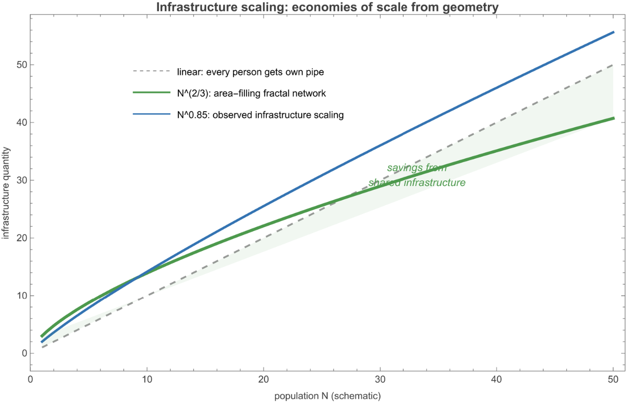
Figure 3.1 Infrastructure scaling: the area between the linear case (each person gets their own pipe) and the fractal case represents the economies of scale from shared infrastructure. The observed β ≈ 0.85 falls between these bounds.
2/3
N
3.2 Socioeconomic output: social network density
3.2 Socioeconomic output: social network density
The key idea. Innovation, wealth creation, cultural production, and (regrettably) crime all arise from human interactions. The rate of these outputs depends on how many effective interactions each person has. In a complete graph of N people, the number of possible pairwise interactions is N(N−1)/2 ∝ N². But people don't interact with everyone in the city — they interact with those they encounter.
Bettencourt's insight: the effective number of interactions per person scales with the local population density. In a city of area A, the average person encounters others at a rate proportional to N/A. Since A ∝ with α < 1, the density N/A ∝ grows with city size. The total socioeconomic output is then:
α
N
1−α
N
Y∝N·∝
N
A
2-α
N
With α = 5/6, this gives = 2 − 5/6 = 7/6 ≈ 1.167. Across the urban-scaling literature the observed socioeconomic exponents (GDP, wages, innovation, crime) cluster around 1.1–1.3, broadly consistent with this prediction — and, as §5 shows, so do our own UK figures for GVA and business density.
β
soc
The symmetry. Note that the infrastructure exponent and the socioeconomic exponent are related by:
β
infra
β
soc
αd
2
α(d-2)
2
For d = 2 (space-filling network), this sum is exactly 2, giving + = 2. Since both are measured relative to the linear case (β = 1), the deviations are symmetric: (1 − ) = ( − 1) = 1/6 ≈ 0.167. This is a strong, non-trivial prediction of the theory.
β
infra
β
soc
β
infra
β
soc
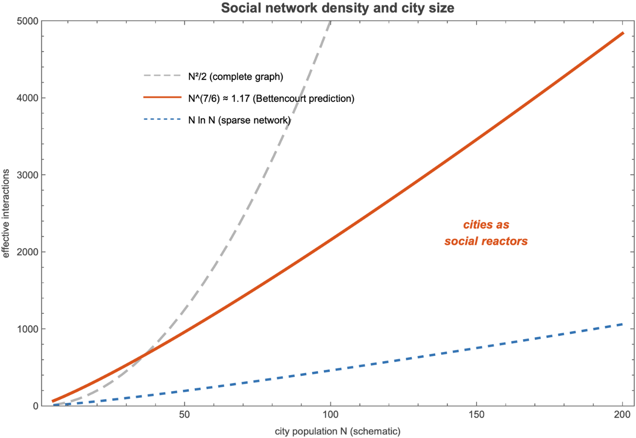
Figure 3.2 Social network density versus city size. The complete-graph scaling (N², grey dashed) is an upper bound; the sparse-network scaling (N ln N, blue dashed) is a lower bound. Bettencourt's prediction ( ≈ , orange solid) falls between the two, reflecting the constraint that interactions are limited by spatial density.
7/6
N
1.17
N
3.3 The Bettencourt unified model (2013)
3.3 The Bettencourt unified model (2013)
The full 2013 model adds one more ingredient: an equilibrium condition. People choose where to live by balancing the benefits of urban agglomeration (access to jobs, services, social interactions) against the costs of commuting (time, transport). The full model imposes this balance on the margin; stated heuristically, at the equilibrium size benefit and cost track each other:
benefit(N)-cost(N)=const
4. Real data: 46 UK cities from open government
4. Real data: 46 UK cities from open government
Everything below runs on real, openly-licensed data. The companion package ScalingLawsCities.wl (next to this notebook) bundles the dataset and the analysis functions, so the notebook is self-contained: evaluate any cell to reproduce its figure. Load it once:
The dataset covers 46 UK cities, each taken as its principal local authority district (the unit at which UK official statistics are actually published), except London, which is the sum of its 33 local authorities. Every series is joined by ONS GSS code. The metrics:
• Population — ONS mid-year population estimates (via the Nomis API).
• GVA (gross value added, £m) — ONS Regional GVA (balanced) by local authority, current prices, 2016 (the latest year in that published release). Economic output.
• Businesses — ONS UK Business Counts (local units, all industries). Enterprise density.
• Jobs — ONS Business Register and Employment Survey (total employment).
• Road length (km of major roads) — DfT Road Lengths in Great Britain (table RDL0202). Physical infrastructure.
• Recorded crime — Home Office / ONS police-recorded crime by local authority, year ending March 2024. Social pathology.
Coverage and vintage. Population, GVA, land area and road length are UK-wide; the business-count, employment and recorded-crime series are published for England and Wales only, so the Scottish cities (Edinburgh, Aberdeen, Dundee) carry a blank there and appear in those fits with a slightly smaller sample. The GVA release is dated 2016 while population, businesses and jobs are the latest available and road length is 2025, so per-capita comparisons mix years a few apart — adequate for the broad scaling pattern, but a reason to read any individual city's residual as indicative rather than exact.
The full dataset is the package's cityData[] (here, the 12 largest; “–” marks a value not available for that city):
Acknowledgement & licence. The population, GVA, business, employment and land-area figures are produced by the Office for National Statistics; recorded crime by the Home Office; road lengths by the Department for Transport; coordinates from the Wolfram Knowledgebase. The official statistics contain public sector information licensed under the Open Government Licence v3.0. Exact datasets, periods and source URLs are listed in data/SOURCES.md and the fetch is fully reproducible via wolfram/fetch_city_data.wls.
A note on geography. Local-authority boundaries are not perfect functional cities, and — as the UK scaling literature stresses (Arcaute 2015; Cottineau 2017) — estimated exponents are sensitive to exactly how a city is delineated. We use the LAD as a transparent, reproducible unit and read the exponents as robust in direction rather than precise to the third decimal.
5. Fitting the power laws
5. Fitting the power laws
For each metric we fit ln Y = ln Y₀ + β ln N by ordinary least squares across the 46 cities, and report β with its 95% confidence interval, R², and a test of H₀: β = 1 (is the scaling distinguishable from linear?). The package does this in one call: scalingFit[col] returns an association with beta, ci, bootstrapCI, pValue, r2 and the per-city residuals, and scalingScatter[col, label] draws the log-log fit with a β = 1 reference line.
5.1 Infrastructure: road length (sublinear)
5.1 Infrastructure: road length (sublinear)
Figure 5.1 Major-road length vs population (log-log), with the fitted power law (blue) and a β=1 reference line (grey).
5.2 Employment: close to linear
5.2 Employment: close to linear
Figure 5.2 Total employment vs population (log-log).
β = 1.10 [analytic 95% CI: 0.99, 1.21; bootstrap CI: 0.96, 1.26], R² = 0.90. Employment tracks population almost one-for-one, with a hint of superlinearity (the interval just includes 1). Jobs behave much like an individual-needs quantity — every working resident is roughly one job's worth of activity — so this sits near the linear baseline, between the sublinear infrastructure and the clearly superlinear economic metrics below.
5.3 Socioeconomic outputs: GVA, businesses, and crime
5.3 Socioeconomic outputs: GVA, businesses, and crime
Figure 5.3 Gross value added vs population (log-log).
Figure 5.4 Business counts (local units) vs population.
Businesses: β = 1.14 [analytic 95% CI: 1.05, 1.24; bootstrap CI: 0.95, 1.19], R² = 0.94. This is the cleanest fit — population alone explains 94% of the variation — and the strongest analytic signal (p = 0.003): larger cities carry disproportionately more enterprises per head, the agglomeration of firms that is the engine of the social-reactor effect. Like GVA, its bootstrap and leave-London intervals reach down toward 1, so the superlinearity is clearest for the full UK system, primate city included.
The dark side. The same density of interaction that makes big cities productive also makes them less safe. Recorded crime (police-recorded offences, year ending March 2024) scales mildly superlinearly in point estimate:
Figure 5.5 Police-recorded crime vs population (log-log).
Figure 5.6 The five scaling exponents with 95% confidence intervals. The economic metrics (GVA, businesses) sit clearly and significantly above β=1; crime and employment straddle it; major roads sit below in point estimate but with an interval that still touches 1. So the superlinear regime is recovered decisively, the sublinear one only directionally — the pattern the theory predicts, with the strength the sample allows.
Two checks keep the inference honest. First, the package also computes a pairs-bootstrap interval for each exponent (B = 999), which is wider for the London-levered economic fits than the analytic Student-t interval. Second, diagnosticTable[] reports residual normality and a Breusch-Pagan-style check for changing residual variance:
The diagnostic headline is modest. GVA residuals are non-normal by Shapiro-Wilk (p ≈ 0.017), mainly because of a few high-value residual cities, while the other metrics do not reject normality at 5%. The Breusch-Pagan-style tests do not flag heteroscedasticity for any metric (all p > 0.25), so the main caution is leverage and tail shape rather than visibly increasing residual spread.
5.4 A structural test: area and density
5.4 A structural test: area and density
Figure 5.7 Land area vs population (log-log). The fitted slope is the area-population exponent the theory predicts to be 5/6.
6. Residual analysis: which cities deviate and why
6. Residual analysis: which cities deviate and why
The fit predicts each city's output from its population; the residual — the gap between prediction and observation — flags which cities systematically over- or under-perform. residualPlot[col, label] plots the standardised residuals and labels everything beyond ±2σ:
Figure 6.1 Standardised residuals from the GVA scaling law; cities beyond ±2σ are labelled.
GVA over-performers — cities producing far more economic output than their size predicts:
• Aberdeen (+2.7σ, the single largest over-performance in the dataset) — the North Sea oil-and-gas economy concentrates enormous value in a city of about 230,000 people.
• Reading (+2.3σ) and Milton Keynes (+2.1σ) — M4-corridor and new-town business and technology clusters.
• Edinburgh (+1.6σ, just inside the 2σ band so unlabelled on the plot above) — Scotland's financial and professional-services centre.
GVA under-performers — Wigan, Dudley, Tameside, Bolton and Rochdale (all about −1.1 to −1.4σ): post-industrial boroughs of Greater Manchester and the West Midlands that lost their heavy-industry base and have not fully transitioned to the knowledge economy.
The pattern is even tighter for business density, the most decisively superlinear metric:
Figure 6.2 Standardised residuals from the business-count scaling law.
Mapped geographically, the residuals trace the UK's economic divide. residualMap[] draws each city's GVA residual on the real coastline:
Figure 6.3 GVA scaling residuals on the UK coastline. Blue: above prediction (knowledge- and energy-economy cities of the South, East and the two Scottish centres Aberdeen and Edinburgh); red: below prediction (post-industrial cities of the North and Midlands). The North-South divide is striking.
7. The London effect
7. The London effect
London dominates the dataset: aggregated across its 33 local authorities it has about 9.1 million people — more than seven times the next-largest city (Birmingham, 1.18 million) — and it sits at the extreme right of every log-log plot. The natural worry is whether this one point drives the fits.
It has high leverage (it is far out along the population axis), but it lies close to the fitted lines rather than far off them: its GVA and business counts are about what the scaling law predicts for a city of nine million. Re-fitting without London leaves the direction of the point estimates intact but weakens the economic evidence: GVA becomes β ≈ 1.05, businesses β ≈ 1.05, jobs β ≈ 1.11, and major roads β ≈ 0.85. In that sense London is a high-leverage confirmation of the whole-system scaling pattern, and the London-free sample should be read as directionally consistent but much less precise.
London in international context. Bettencourt et al. (2007) found that the largest city in each country typically sits a few tenths of a log-unit above the regression line, reflecting the extra pull of a national capital and global financial centre. London is consistent with that pattern: a primate city, but one that still obeys the same exponent as the rest of the system rather than breaking it.
8. Comparison with international results
8. Comparison with international results
How do the UK exponents compare with those found in other countries?
The prediction-observation match is good. Two regimes come through clearly: GVA and business counts are significantly superlinear (β = 1.15 and 1.14, both with p < 0.05), and major roads are sublinear in point estimate (β = 0.86). Employment (1.10) sits at the linear baseline. So from real, independent UK data we recover the theory's superlinear regime decisively — the agreement on the economic exponent (1.15) is the headline result — while the sublinear-infrastructure regime is confirmed in direction but, with 46 cities and a major-roads-only measure, not sharply separated from linear. One clean regime and two suggestive ones is an honest reading of the evidence.
9. Policy implications
9. Policy implications
What the scaling laws tell us about cities. The scaling framework has several concrete implications for urban policy:
1. Big cities are more efficient per capita. The sublinear infrastructure exponent (β ≈ 0.86) means large cities need proportionally less road per person. This is an engineering efficiency argument for agglomeration: consolidating population into fewer, larger cities lowers the per-capita cost of infrastructure — for the UK, roughly a 9% per-capita saving each time a city doubles in size.
2. Growth concentrates economically. The superlinear exponents (GVA and businesses near β = 1.15) mean output and enterprise grow faster than population: a city twice the size is more than twice as productive per its own scale. That is good for national output but tends to widen regional inequality, concentrating value in the largest and most successful cities. The policy lever is not to shrink cities — that would forfeit the agglomeration gains — but to help smaller cities climb the curve.
3. The scaling residuals diagnose city performance. A city above the line over-performs for its size; one below under-performs. The residual is a size-adjusted benchmark that strips out the population effect. For the UK it paints a stark North-South / post-industrial divide: energy and knowledge cities (Aberdeen, Reading, Milton Keynes, Edinburgh) over-perform on GVA, while post-industrial boroughs (Wigan, Dudley, Tameside, Bolton, Rochdale) sit about 1–1.4 standard deviations below.
4. The scaling framework sets expectations. Before judging a city we need to know what to expect for its size. A city of 200,000 is not “failing” because it produces less GVA than one of 2,000,000; the scaling law says how much less to expect. For setting regeneration targets the goal is not to match London but to close the gap to the line — a far more realistic and size-fair benchmark.
10. Conclusion
10. Conclusion
We set out to test a simple but radical idea on real UK data: that a city is not a big village but a different kind of object, one whose properties bend predictably with size. Across 46 cities — built entirely from open government statistics — the bend is real and it points where the theory predicts. Major-road length scales sublinearly (β ≈ 0.86) — infrastructure shared, not replicated. Employment tracks population close to linearly (β ≈ 1.10). And GVA and business density scale clearly superlinearly (β ≈ 1.15 and 1.14, both significant) — the signature of the social-reactor effect, the density of human contact that makes bigger cities disproportionately more productive.
The headline is that the real UK economic exponent lands almost exactly on Bettencourt's canonical 1.15 — a genuinely independent confirmation, from a different country and different data, of a number derived from first principles. We have also been honest about the limits: with 46 cities the infrastructure interval is wide (sublinear in point estimate, not sharply distinguishable from linear), and the exponents shift with how a city's boundary is drawn, a caveat the UK boundary literature (Arcaute 2015; Cottineau 2017) makes vivid — which is why we read them as robust in direction rather than precise to the decimal.
What survives is a useful lens rather than a deterministic law. The residuals — who beats their size and who falls short — trace the UK's economic geography sharply: a knowledge economy concentrated in the South and East, a post-industrial belt across the North and Midlands still closing the gap. Read this way, scaling laws are less a verdict on cities than a fair yardstick: they tell us what to expect from a place of a given size, so we can ask the more interesting question — why some places beat the line, and what it would take for others to.
11. References
11. References
Bettencourt, L. M. A., Lobo, J., Helbing, D., Kühnert, C., & West, G. B. (2007). Growth, innovation, scaling, and the pace of life in cities. Proceedings of the National Academy of Sciences 104(17), 7301–7306. [The founding empirical paper of urban scaling.]
Bettencourt, L. M. A. (2013). The origins of scaling in cities. Science 340(6139), 1438–1441. [The theoretical derivation from first principles.]
West, G. B. (2017). Scale: The Universal Laws of Life, Growth, and Death in Organisms, Cities, and Companies. Penguin Press. [Popular-science treatment.]
Batty, M. (2013). The New Science of Cities. MIT Press. [Broader context of urban complexity.]
Zipf, G. K. (1949). Human Behavior and the Principle of Least Effort. Addison-Wesley. [The original city-size distribution.]
Arcaute, E., Hatna, E., Ferguson, P., Youn, H., Johansson, A., & Batty, M. (2015). Constructing cities, deconstructing scaling laws. Journal of the Royal Society Interface 12(102), 20140745. [UK-specific analysis showing sensitivity to city boundary definitions.]
Cottineau, C., Hatna, E., Arcaute, E., & Batty, M. (2017). Diverse cities or the systematic paradox of urban scaling laws. Computers, Environment and Urban Systems 63, 80–94. [Detailed UK analysis with multiple boundary definitions.]
Leitao, J. C., Miotto, J. M., Gerlach, M., & Altmann, E. G. (2016). Is this scaling nonlinear? Royal Society Open Science 3(7), 150649. [Methodological critique of urban scaling analyses.]
Oliveira, E. A., Andrade, J. S., & Makse, H. A. (2014). Large cities are less green. Scientific Reports 4, 4235. [Extension to environmental metrics.]
Bettencourt, L. M. A., & Lobo, J. (2016). Urban scaling in Europe. Journal of the Royal Society Interface 13(116), 20160005. [European cross-country comparison.]
12. Reproducibility
12. Reproducibility
Everything in this notebook is reproducible. The figures are produced live by the companion package ScalingLawsCities.wl (kept next to the notebook), which embeds the dataset, so you can re-run any cell as-is. The full pipeline — re-fetching the raw open data, rebuilding the package and the notebook — is pure Wolfram Language and lives in the public repository github.com/mthiel74/scalinglawsincities (https://github.com/mthiel74/scalinglawsincities):
# 1. Fetch the real open data from ONS / DfT into data/uk_cities.csv
wolframscript -file wolfram/fetch_city_data.wls
# 2. Render all static figures
wolframscript -file wolfram/run_all.wls
# 3. Rebuild the companion package and the notebook
wolframscript -file community/build_package.wls
wolframscript -file community/build_notebook.wls
wolframscript -file wolfram/fetch_city_data.wls
# 2. Render all static figures
wolframscript -file wolfram/run_all.wls
# 3. Rebuild the companion package and the notebook
wolframscript -file community/build_package.wls
wolframscript -file community/build_notebook.wls
Data acknowledgement. Population, gross value added, business counts and employment are produced by the Office for National Statistics (accessed via the Nomis API and ONS dataset downloads); major-road lengths by the Department for Transport (table RDL0202); city coordinates from the Wolfram Knowledgebase. The official statistics contain public sector information licensed under the Open Government Licence v3.0. Exact datasets, reference periods and source URLs are in data/SOURCES.md.
Generated on June 10, 2026 with Wolfram Language 15.0.
CITE THIS NOTEBOOK
CITE THIS NOTEBOOK
Cities as social reactors: Bettencourt 2013 urban scaling replicated across 46 UK cities
by Marco Thiel
Wolfram Community, STAFF PICKS, June 10, 2026
https://community.wolfram.com/groups/-/m/t/3731000
by Marco Thiel
Wolfram Community, STAFF PICKS, June 10, 2026
https://community.wolfram.com/groups/-/m/t/3731000