Smith’s Graphical Techniques for Second-Order Models
Authors: Housam Binous and Ahmed Bellagi
Smith’s Graphical Techniques for Second-Order Models
Authors: Housam Binous and Ahmed Bellagi
Authors: Housam Binous and Ahmed Bellagi
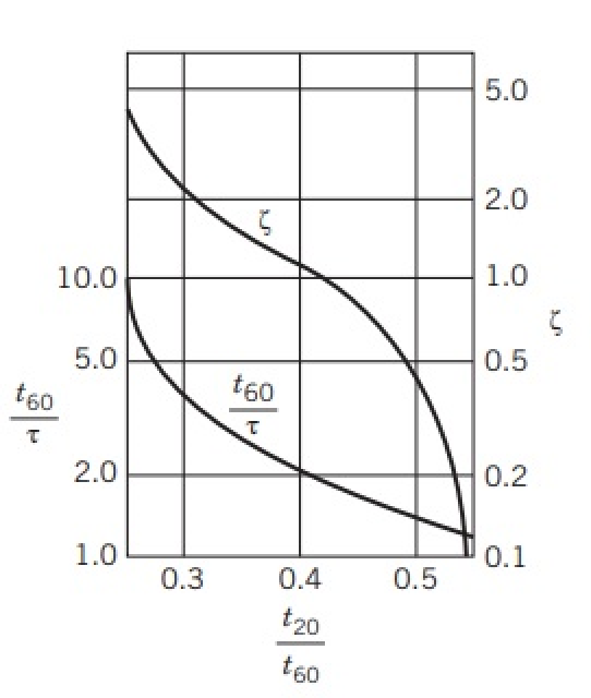
Consider an overdamped or underdamped model with a unit step response represented by , where and ζ ( or ) are the time constant and the damping coefficient, respectively. It is possible to use the step-response data in order to obtain approximate values for and . Such a method was developed by Smith [1] and uses the times at which the normalized response reaches 20% and 60% (at times and . Indeed, the ratio / gives (blue dashed curve) and /τ (green dashed curve).These computed curves are successfully compared to their counterparts obtained by digitizing Fig. 7-7 given in Ref. 2 page 111 (digitized data are indicated by the red dots).References :[1] C. L. Smith, Digital Computer Process Control, Scranton: Intext Educational Publishers, 1972. [2] D. E. Seborg, T. F. Edgar, D. A. Mellichamp, and F. J. Doyle III, Process Dynamics and Control, 4th ed., New York: Wiley, 2017.
U×G=×1+2τζs+1
1
s
2
τ
2
s
τ
ζ>1
ζ<1
τ
ζ
t
20
t
60
)
t
20
t
60
ζ
t
60
In[]:=
y[t_,ζ_,τ_]:=InverseLaplaceTransform[1/s1/(τ^2s^2+2τζs+1),s,t]
In[]:=
τ=1;
In[]:=
LaunchKernels[]
Out[]=
KernelObject,KernelObject,KernelObject,KernelObject

In[]:=
tbl=Parallelize@Table[{(t/.FindRoot[y[t,ζ,τ]0.2,{t,τ/2}])/(t/.FindRoot[y[t,ζ,τ]0.6,{t,τ}]),(t/.FindRoot[y[t,ζ,τ]0.6,{t,τ}])/τ,ζ},{ζ,0.1,5,0.05}];
In[]:=
tbl2=tbl//Chop
Out[]=
{{0.543322,1.21112,0.1},{0.537165,1.239,0.15},{0.530819,1.26831,0.2},{0.524283,1.29914,0.25},{0.517554,1.3316,0.3},{0.510633,1.3658,0.35},{0.503521,1.40187,0.4},{0.49622,1.43992,0.45},{0.488737,1.48008,0.5},{0.48108,1.52248,0.55},{0.473261,1.56725,0.6},{0.465296,1.6145,0.65},{0.457203,1.66436,0.7},{0.449008,1.71693,0.75},{0.440739,1.77229,0.8},{0.432429,1.83049,0.85},{0.424116,1.89158,0.9},{0.41584,1.95554,0.95},{0.407646,2.02231,1.},{0.399578,2.09182,1.05},{0.391678,2.16394,1.1},{0.383989,2.23849,1.15},{0.376546,2.31529,1.2},{0.369382,2.39411,1.25},{0.362521,2.47475,1.3},{0.355981,2.55696,1.35},{0.349771,2.64055,1.4},{0.343897,2.7253,1.45},{0.338357,2.81104,1.5},{0.333144,2.89762,1.55},{0.32825,2.98489,1.6},{0.323661,3.07274,1.65},{0.319363,3.16108,1.7},{0.315342,3.24982,1.75},{0.311582,3.3389,1.8},{0.308066,3.42827,1.85},{0.30478,3.51788,1.9},{0.301708,3.6077,1.95},{0.298836,3.6977,2.},{0.29615,3.78785,2.05},{0.293637,3.87813,2.1},{0.291286,3.96853,2.15},{0.289084,4.05903,2.2},{0.287021,4.14962,2.25},{0.285088,4.24029,2.3},{0.283274,4.33103,2.35},{0.281571,4.42184,2.4},{0.279971,4.5127,2.45},{0.278467,4.60361,2.5},{0.277052,4.69456,2.55},{0.275719,4.78556,2.6},{0.274463,4.8766,2.65},{0.273279,4.96767,2.7},{0.27216,5.05878,2.75},{0.271103,5.14991,2.8},{0.270103,5.24107,2.85},{0.269157,5.33225,2.9},{0.268261,5.42346,2.95},{0.26741,5.51468,3.},{0.266604,5.60593,3.05},{0.265837,5.69719,3.1},{0.265109,5.78847,3.15},{0.264415,5.87977,3.2},{0.263755,5.97108,3.25},{0.263126,6.06241,3.3},{0.262526,6.15374,3.35},{0.261954,6.24509,3.4},{0.261407,6.33645,3.45},{0.260885,6.42782,3.5},{0.260385,6.5192,3.55},{0.259906,6.61059,3.6},{0.259448,6.70199,3.65},{0.259009,6.7934,3.7},{0.258589,6.88482,3.75},{0.258185,6.97624,3.8},{0.257797,7.06767,3.85},{0.257425,7.1591,3.9},{0.257067,7.25055,3.95},{0.256723,7.34199,4.},{0.256392,7.43345,4.05},{0.256073,7.52491,4.1},{0.255766,7.61637,4.15},{0.255471,7.70784,4.2},{0.255186,7.79932,4.25},{0.254911,7.8908,4.3},{0.254646,7.98228,4.35},{0.25439,8.07377,4.4},{0.254142,8.16526,4.45},{0.253904,8.25675,4.5},{0.253673,8.34825,4.55},{0.25345,8.43975,4.6},{0.253234,8.53126,4.65},{0.253025,8.62277,4.7},{0.252823,8.71428,4.75},{0.252628,8.8058,4.8},{0.252438,8.89731,4.85},{0.252254,8.98883,4.9},{0.252076,9.08036,4.95},{0.251904,9.17188,5.}}
In[]:=
TableForm@Join[{{"/","/τ","ζ "}},tbl2]
t
20
t
60
t
60
Out[]//TableForm=
t 20 t 60 | t 60 | ζ |
0.543322 | 1.21112 | 0.1 |
0.537165 | 1.239 | 0.15 |
0.530819 | 1.26831 | 0.2 |
0.524283 | 1.29914 | 0.25 |
0.517554 | 1.3316 | 0.3 |
0.510633 | 1.3658 | 0.35 |
0.503521 | 1.40187 | 0.4 |
0.49622 | 1.43992 | 0.45 |
0.488737 | 1.48008 | 0.5 |
0.48108 | 1.52248 | 0.55 |
0.473261 | 1.56725 | 0.6 |
0.465296 | 1.6145 | 0.65 |
0.457203 | 1.66436 | 0.7 |
0.449008 | 1.71693 | 0.75 |
0.440739 | 1.77229 | 0.8 |
0.432429 | 1.83049 | 0.85 |
0.424116 | 1.89158 | 0.9 |
0.41584 | 1.95554 | 0.95 |
0.407646 | 2.02231 | 1. |
0.399578 | 2.09182 | 1.05 |
0.391678 | 2.16394 | 1.1 |
0.383989 | 2.23849 | 1.15 |
0.376546 | 2.31529 | 1.2 |
0.369382 | 2.39411 | 1.25 |
0.362521 | 2.47475 | 1.3 |
0.355981 | 2.55696 | 1.35 |
0.349771 | 2.64055 | 1.4 |
0.343897 | 2.7253 | 1.45 |
0.338357 | 2.81104 | 1.5 |
0.333144 | 2.89762 | 1.55 |
0.32825 | 2.98489 | 1.6 |
0.323661 | 3.07274 | 1.65 |
0.319363 | 3.16108 | 1.7 |
0.315342 | 3.24982 | 1.75 |
0.311582 | 3.3389 | 1.8 |
0.308066 | 3.42827 | 1.85 |
0.30478 | 3.51788 | 1.9 |
0.301708 | 3.6077 | 1.95 |
0.298836 | 3.6977 | 2. |
0.29615 | 3.78785 | 2.05 |
0.293637 | 3.87813 | 2.1 |
0.291286 | 3.96853 | 2.15 |
0.289084 | 4.05903 | 2.2 |
0.287021 | 4.14962 | 2.25 |
0.285088 | 4.24029 | 2.3 |
0.283274 | 4.33103 | 2.35 |
0.281571 | 4.42184 | 2.4 |
0.279971 | 4.5127 | 2.45 |
0.278467 | 4.60361 | 2.5 |
0.277052 | 4.69456 | 2.55 |
0.275719 | 4.78556 | 2.6 |
0.274463 | 4.8766 | 2.65 |
0.273279 | 4.96767 | 2.7 |
0.27216 | 5.05878 | 2.75 |
0.271103 | 5.14991 | 2.8 |
0.270103 | 5.24107 | 2.85 |
0.269157 | 5.33225 | 2.9 |
0.268261 | 5.42346 | 2.95 |
0.26741 | 5.51468 | 3. |
0.266604 | 5.60593 | 3.05 |
0.265837 | 5.69719 | 3.1 |
0.265109 | 5.78847 | 3.15 |
0.264415 | 5.87977 | 3.2 |
0.263755 | 5.97108 | 3.25 |
0.263126 | 6.06241 | 3.3 |
0.262526 | 6.15374 | 3.35 |
0.261954 | 6.24509 | 3.4 |
0.261407 | 6.33645 | 3.45 |
0.260885 | 6.42782 | 3.5 |
0.260385 | 6.5192 | 3.55 |
0.259906 | 6.61059 | 3.6 |
0.259448 | 6.70199 | 3.65 |
0.259009 | 6.7934 | 3.7 |
0.258589 | 6.88482 | 3.75 |
0.258185 | 6.97624 | 3.8 |
0.257797 | 7.06767 | 3.85 |
0.257425 | 7.1591 | 3.9 |
0.257067 | 7.25055 | 3.95 |
0.256723 | 7.34199 | 4. |
0.256392 | 7.43345 | 4.05 |
0.256073 | 7.52491 | 4.1 |
0.255766 | 7.61637 | 4.15 |
0.255471 | 7.70784 | 4.2 |
0.255186 | 7.79932 | 4.25 |
0.254911 | 7.8908 | 4.3 |
0.254646 | 7.98228 | 4.35 |
0.25439 | 8.07377 | 4.4 |
0.254142 | 8.16526 | 4.45 |
0.253904 | 8.25675 | 4.5 |
0.253673 | 8.34825 | 4.55 |
0.25345 | 8.43975 | 4.6 |
0.253234 | 8.53126 | 4.65 |
0.253025 | 8.62277 | 4.7 |
0.252823 | 8.71428 | 4.75 |
0.252628 | 8.8058 | 4.8 |
0.252438 | 8.89731 | 4.85 |
0.252254 | 8.98883 | 4.9 |
0.252076 | 9.08036 | 4.95 |
0.251904 | 9.17188 | 5. |