Version 13.1 of Mathematica now has the function built in. This function allows you to generate graphs corresponding to the skeletons of Goldberg polyhedra, which are more popularly known to be the forms taken by the allotropes of carbon known as fullerenes (a.k.a. buckyballs). The most popular among the fullerenes is , whose skeleton corresponds to the skeleton of the truncated icosahedron.
C
60
Here is a representation of the usual buckyball:
In[]:=
bucky=BuckyballGraph[]
Out[]=

We can easily verify that it is the 1-skeleton of the truncated icosahedron:
In[]:=
IsomorphicGraphQ[bucky,MeshConnectivityGraph[UniformPolyhedron["TruncatedIcosahedron"],0]]
Out[]=
True
C
60
In[]:=
Out[]=

It is interesting to see if we can make a molecular model of a fullerene from its corresponding graph. To do this, we need a way to find out how to appropriately distribute the single and double bonds in the molecular representation. (At this juncture, I should say that in reality, the electrons in an actual fullerene molecule are delocalized, but we are explicitly assigning single and double bonds (a.k.a. a Kekule form) for modeling purposes.)After some preprocessing with to canonicalize the indexing of the vertices, it turns out that one only needs to find an independent edge set (i.e. a matching) for the graph, which can be done through the built-in function :
In[]:=
bucky=IndexGraph[bucky];el=Sort/@EdgeList[bucky];dbl=Sort/@FindIndependentEdgeSet[bucky]
Out[]=
{13,25,49,610,741,824,1113,1216,1420,1529,1743,1832,1942,2123,2226,2537,2738,2857,3033,3136,3450,3539,4058,4447,4546,4859,4960,5152,5355,5456}
We can then use this matching to generate the list of all the carbon-carbon bonds in the buckyball:
In[]:=
bonds=Join[Bond[{##},"Single"]&@@@Complement[el,dbl],Bond[{##},"Double"]&@@@dbl]
Out[]=
{Bond[{1,2},Single],Bond[{1,4},Single],Bond[{2,6},Single],Bond[{3,7},Single],Bond[{3,8},Single],Bond[{4,10},Single],Bond[{5,21},Single],Bond[{5,24},Single],Bond[{6,26},Single],Bond[{7,51},Single],Bond[{8,53},Single],Bond[{9,41},Single],Bond[{9,42},Single],Bond[{10,47},Single],Bond[{11,12},Single],Bond[{11,14},Single],Bond[{12,15},Single],Bond[{13,17},Single],Bond[{13,18},Single],Bond[{14,19},Single],Bond[{15,32},Single],Bond[{16,20},Single],Bond[{16,34},Single],Bond[{17,52},Single],Bond[{18,54},Single],Bond[{19,43},Single],Bond[{20,49},Single],Bond[{21,22},Single],Bond[{22,25},Single],Bond[{23,27},Single],Bond[{23,28},Single],Bond[{24,28},Single],Bond[{25,45},Single],Bond[{26,48},Single],Bond[{27,37},Single],Bond[{29,30},Single],Bond[{29,31},Single],Bond[{30,34},Single],Bond[{31,35},Single],Bond[{32,36},Single],Bond[{33,39},Single],Bond[{33,46},Single],Bond[{35,38},Single],Bond[{36,58},Single],Bond[{37,39},Single],Bond[{38,40},Single],Bond[{40,57},Single],Bond[{41,43},Single],Bond[{42,44},Single],Bond[{44,49},Single],Bond[{45,48},Single],Bond[{46,50},Single],Bond[{47,59},Single],Bond[{50,60},Single],Bond[{51,53},Single],Bond[{52,54},Single],Bond[{55,56},Single],Bond[{55,57},Single],Bond[{56,58},Single],Bond[{59,60},Single],Bond[{1,3},Double],Bond[{2,5},Double],Bond[{4,9},Double],Bond[{6,10},Double],Bond[{7,41},Double],Bond[{8,24},Double],Bond[{11,13},Double],Bond[{12,16},Double],Bond[{14,20},Double],Bond[{15,29},Double],Bond[{17,43},Double],Bond[{18,32},Double],Bond[{19,42},Double],Bond[{21,23},Double],Bond[{22,26},Double],Bond[{25,37},Double],Bond[{27,38},Double],Bond[{28,57},Double],Bond[{30,33},Double],Bond[{31,36},Double],Bond[{34,50},Double],Bond[{35,39},Double],Bond[{40,58},Double],Bond[{44,47},Double],Bond[{45,46},Double],Bond[{48,59},Double],Bond[{49,60},Double],Bond[{51,52},Double],Bond[{53,55},Double],Bond[{54,56},Double]}
From that, we can now generate the corresponding buckyball molecule. To ease things a bit, we also supply the coordinates of the graph embedding as an initial approximation to the 3D coordinates of the buckyball:
In[]:=
bmol=Molecule[ConstantArray[Atom["C"],VertexCount[bucky]],bonds,AtomCoordinates->QuantityArray[1.6GraphEmbedding[bucky],"Angstroms"]]
Out[]=
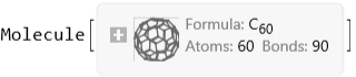
We then recompute the coordinates corresponding to a configuration with minimal force-field energy, using :
In[]:=
bmol=MoleculeModify[bmol,"EnergyMinimizeAtomCoordinates"]
Out[]=
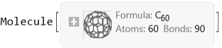
After all that work, we can finally visualize the result:
In[]:=
MoleculePlot3D[bmol]
Out[]=

In[]:=
ServiceExecute["PubChem","CompoundDescription",{"InChIKey"->MoleculeValue[bmol,"InChIKey"]["ExternalID"]}]
Out[]=
This approach can also be used to make other fullerenes. For instance, we can also make the fullerene corresponding to the skeleton of the chamfered dodecahedron:
In[]:=
ch=IndexGraph[BuckyballGraph[1,"I"]];el=Sort/@EdgeList[ch];dbl=Sort/@FindIndependentEdgeSet[ch];cmol=MoleculeModify[Molecule[ConstantArray[Atom["C"],VertexCount[ch]],Join[Bond[{##},"Single"]&@@@Complement[el,dbl],Bond[{##},"Double"]&@@@dbl],AtomCoordinates->QuantityArray[1.6GraphEmbedding[ch],"Angstroms"]],"EnergyMinimizeAtomCoordinates"]
Visualize the structure: