Cocurrent-Flow Model for Gas Separation by Membranes Authors: Housam Binous and Ahmed Bellagi
Cocurrent-Flow Model for Gas Separation by Membranes Authors: Housam Binous and Ahmed Bellagi
reference : H . Binous, Gas Permeation Computations with Mathematica®, Chemical Engineering Education, 40 (2), pp . 140 - 144, 2006.
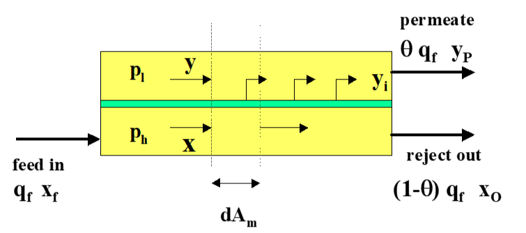
We compute the permeate and residue compositions obtained using a membrane separation module . Membrane area is also computed . Feed is air and is considered as a binary mixture . Cocurrent-flow mixing model is used . We use the shooting technique in order to determine the surface area of the separation module.
Reference:
C. J. Geankoplis, Transport Processes and Unit Operations, 3rd edition, Prentice Hall, 1993.
W. P. Walawender and S. A. Stern, Separation Science, 7 (5), pp. 553-584, 1972.
C. J. Geankoplis, Transport Processes and Unit Operations, 3rd edition, Prentice Hall, 1993.
W. P. Walawender and S. A. Stern, Separation Science, 7 (5), pp. 553-584, 1972.
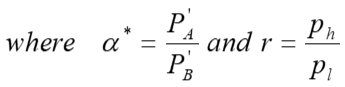
The separation factor for this binary mixture (components A and B) that we want to separate by membrane permeation is ==10.
*
α
P'
A
P'
B
In[]:=
α=10;
The pressure of the feed side is =190cmHgwhile =19 cmHg is the pressure on the permeate side.
p
h
p
l
In[]:=
p
l
In[]:=
p
h
Stage cut is equal to θ=0.2. The material balance is given by the following equation:

In[]:=
θ=0.2;
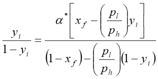
Mole fraction at end of separation module is .It is related to by the following equation:
y
i
x
f
In[]:=
sol=Solve[y/(1-y)(α((xf-/y)/(1-xf-/(1-y)))),y]
p
l
p
h
p
l
p
h
Out[]=
y19+90xf-19+90xf+
1
18
361-180xf+8100
,y2
xf
1
18
361-180xf+8100
2
xf
In[]:=
yi=y/.sol[[1]];
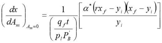
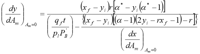
t= 2.54 cm is membrane thickness. =(1-θ)is reject out flow rate. =1(STP)/s is feed flow rate. =50 (STP)cm(scmHg)is the permeability of component B. Governing equations for mole fraction x and y in the reject and permeate sides are given by:
-3
10
q
O
q
f
q
f
6
10
3
cm
P'
B
-10
10
3
cm
2
cm


L'Hôpital rule gives the derivatives as 0.
A
m
In[]:=
q
f
In[]:=
t=2.54 10^-3;
In[]:=
P'
B
In[]:=
xf=0.209;
In[]:=
eq1=D[x[],{,1}]If[0,Evaluate[()/(t)α(xf/-yi)(xf-yi)/yi/.t->2.5410^-3/.->190/.->19/.α->10/.->5010^-10/.->810^5],Evaluate[()/(t)(x[]-y[])/(y[]-xf)((1-x[])α(/x[]-y[])-x[](/(1-x[])-(1-y[])))/.t->2.5410^-3/.->190/.->19/.α->10/.->5010^-10/.->810^5]];
A
m
A
m
A
m
p
l
P'
B
q
f
p
h
p
l
p
h
p
l
P'
B
q
f
p
l
P'
B
q
f
A
m
A
m
A
m
A
m
p
h
p
l
A
m
A
m
A
m
p
h
p
l
A
m
A
m
p
h
p
l
P'
B
q
f
In[]:=
eq2=D[y[],{,1}]If[0,Evaluate[(xf-yi)/(α-yi(α-1))/((t)/()-((xf-yi)/(()/(t)α(xf/-yi)(xf-yi)/yi))((α-1)(2yi-/xf-1)-/))/.t->2.5410^-3/.->190/.->19/.α->10/.->5010^-10/.->810^5],Evaluate[()/(t)(x[]-y[])/(x[]-xf)((1-y[])α(/x[]-y[])-y[](/(1-x[])-(1-y[])))/.t->2.5410^-3/.->190/.->19/.α->10/.->5010^-10/.->810^5]];
A
m
A
m
A
m
p
h
p
l
q
f
p
l
P'
B
p
l
P'
B
q
f
p
h
p
l
p
h
p
l
p
h
p
l
p
h
p
l
P'
B
q
f
p
l
P'
B
q
f
A
m
A
m
A
m
A
m
p
h
p
l
A
m
A
m
A
m
p
h
p
l
A
m
A
m
p
h
p
l
P'
B
q
f
In[]:=
eq3=y[0]yi;
In[]:=
myODEsoln[Ω_]:=NDSolve[{eq1,eq2,eq3,x[0]xf},{x[],y[]},{,0,Ω}]
A
m
A
m
A
m
Use FindRoot to compute surface area of the separation module. Surface area must verify
thematerialbalance.
In[]:=
Off[InterpolatingFunction::dmval]
In[]:=
Off[NDSolve::mxst]
In[]:=
Off[General::spell1]
In[]:=
xend[Ω_?NumericQ]:=Flatten[(x[]/.myODEsoln[Ω])/.Ω]yend[Ω_?NumericQ]:=Flatten[(y[]/.myODEsoln[Ω])/.Ω]=FindRoot[0.2yend[Ω]+0.8xend[Ω]xf,{Ω,3.10^8,5.10^8},MaxIterations1000]
A
m
A
m
A
m
A
m
P
sol
Out[]=
{Ω2.95525×}
8
10
Surface area is equal to 2.95525 .
8
10
2
cm
In[]:=
P
sol
Out[]=
{Ω2.95525×}
8
10
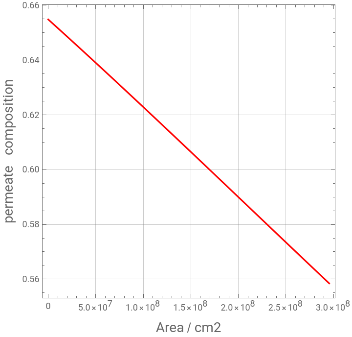
Checking the values of the mole fractions x and y at the entrance and exit of the module. Permeate mole fraction is 0.558456 and reject out mole fraction = 0.121636.
x
O
In[]:=
x[]/.myODEsoln[Ω/.]/.Ω/.
A
m
P
sol
A
m
P
sol
Out[]=
{0.121636}
In[]:=
x[]/.myODEsoln[Ω/.]/.0
A
m
P
sol
A
m
Out[]=
{0.209}
In[]:=
y[]/.myODEsoln[Ω/.]/.Ω/.
A
m
P
sol
A
m
P
sol
Out[]=
{0.558456}
In[]:=
y[]/.myODEsoln[Ω/.]/.0
A
m
P
sol
A
m
Out[]=
{0.654834}
Checking Material Balance: θ +(1-θ) = = 0.209
y
P
x
O
x
f
In[]:=
0.558456 0.2+0.121636 0.8
Out[]=
0.209
Plotting x and y versus surface area of the separation module.
In[]:=
First[y[]/.myODEsoln[Ω/.]]/.area
A
m
P
sol
A
m
Out[]=
InterpolatingFunction[area]


In[]:=
Plot[%,{area,0.001,Ω/.},PlotStyleRGBColor[1,0,0],Frame->True,GridLines->Automatic,AspectRatio->1,FrameLabel->{Style["Area / cm2",14],Style["permeate composition",14]}]
P
sol
Out[]=