This project explores the kinematic behavior of a three-link planar robotic manipulator. Forward kinematics with vector addition is used to determine and control the position of the end effector from specified joint angles, while the FABRIK inverse kinematics algorithm is implemented to compute joint configurations for target positions. By varying link lengths and joint parameters, I analyze their effects on workspace, reachability, and positioning speed. The project demonstrates how computational methods can be applied to optimize robotic manipulator design while providing intuitive visualizations of complex kinematic principles.
Introduction
Introduction
Robotic manipulators are fundamental components of modern automation, enabling machines to perform tasks ranging from industrial assembly to even minimally invasive surgery. A common challenge in robotics is determining how a robotic arm should move so that its end effector reaches a desired target while respecting the fixed lengths of its links and the physical constraints of its joints. This problem is known as inverse kinematics.
This project investigates a planar three-link robotic arm using the Wolfram Language. The arm is first modeled using forward kinematics, where the positions of each joint are determined from the joint angles and link lengths through trigonometric ratios. Building upon this model, the Forward and Backward Reaching Inverse Kinematics (FABRIK) algorithm is implemented to iteratively reposition the arm so that its end effector converges to a specified target.
Unlike analytical inverse kinematics methods that solve systems of equations, FABRIK is a geometric algorithm that repeatedly adjusts joint positions while preserving the lengths of the links. This makes it computationally efficient and well suited for interactive simulations. The primary objective of this computational essay is not only to implement forward and inverse kinematics, but also to investigate how varying the lengths of the robotic arm’s links influences its performance. Metrics such as positioning accuracy (through error analysis), are analyzed to determine how different arm lengths affect the efficiency of the inverse kinematics algorithm.
Legend:
Legend:
◼
P
0
◼
P
1
◼
P
2
◼
P
3
◼
L
1
L
2
L
3
◼
θ
1
θ
2
θ
3
Establishing Concept:
Establishing Concept:
Before implementing the manipulator computationally, it is necessary to establish the mathematical model that lays behind the manipulator. The following section derives the forward kinematics equations used to determine each joint position from the manipulator’s geometry.
A planar robotic manipulator consists of a sequence of rigid links that are connected by rotating joints. In this specific investigation, the manipulator is constrained to move within the Cartesian xy-plane and consists of three links with lengths (L1, L2, L3). The joints rotate, allowing each link to change its orientation while maintaining a constant length.
A planar robotic manipulator consists of a sequence of rigid links that are connected by rotating joints. In this specific investigation, the manipulator is constrained to move within the Cartesian xy-plane and consists of three links with lengths (L1, L2, L3). The joints rotate, allowing each link to change its orientation while maintaining a constant length.
The manipulator originates from a fixed base located at:
P
0
while the remaining joints are represented by:
P
1
P
2
P
3
where represents the end effector.
Unlike independent rotations, each link’s orientation depends upon the rotations of all preceding joints. Consequently,
P
3
Unlike independent rotations, each link’s orientation depends upon the rotations of all preceding joints. Consequently,
◼
Link 1 rotates by ,
θ
1
◼
Link 2 rotates by + ,
θ
1
θ
2
◼
Link 3 rotates by + +
θ
1
θ
2
θ
3
The position of every joint is then obtained through successive vector addition, producing the forward kinematic model of the manipulator.
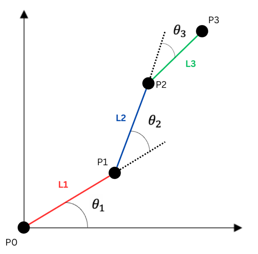
The horizontal and vertical components of each link are obtained using trigonometric ratios:
x = L Cosθ, y = L Sinθ
For the first link, the position of the first joint is therefore:
P
1
L
1
θ
1
L
1
θ
1
Since the second link begins at , its contribution must be added to the coordinates of the first joint. Thus, its orientations is no longer just , but the cumulative angle + .
P
1
θ
2
θ
1
θ
2
P
2
L
1
θ
1
L
2
θ
1
θ
2
L
1
θ
1
L
2
θ
1
θ
2
The same principle applies for the third link. As it originates from , its vector is added to the previous joint’s coordinates, while rotating through the cumulative angle + + . Therefore, is represented as:
P
2
θ
1
θ
2
θ
3
P
3
P
3
L
1
θ
1
L
2
θ
1
θ
2
L
3
θ
1
θ
2
θ
3
L
1
θ
1
L
2
θ
1
θ
2
L
3
θ
1
θ
2
θ
3
Implementing Link Rotation:
Implementing Link Rotation:
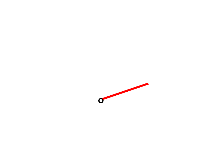
Before constructing the complete three-link manipulator, it is essential to understand the behavior of a single rotating link. This simplified model demonstrates the main geometric transformation that defines the entire robotic arm.
Interactive Visualization of a Single Rotating Link
In[]:=
Manipulate[Graphics[{Rotate[{Red,Rectangle[{0,0},{5,0.2}]},a,{0,0}],{White,EdgeForm[{Black,Thick}],Disk[{0,0},0.2]}},PlotRange->{{-10,12},{-5,10}}],{a,0,Pi},SaveDefinitions->True]
Controls the angle “a” between the bounds (0, π).
Out[]=


Manipulable Three-Link Arm Setup
Manipulable Three-Link Arm Setup
After validating the behavior of a single rotating link, the model is extended to a complete three-link planar manipulator. Rather than treating each link independently, every successive link accumulates the rotation of preceding joints, producing the forward kinematic behavior derived earlier.
Each link is represented as a rectangle that is first translated to the endpoint of the previous link and then rotated about the corresponding joint. This sequence of transformations follows the mathematical foundation of forward kinematics, each joint position being obtained through successive vector addition.
Each link is represented as a rectangle that is first translated to the endpoint of the previous link and then rotated about the corresponding joint. This sequence of transformations follows the mathematical foundation of forward kinematics, each joint position being obtained through successive vector addition.
Interactive Three-Link Planar Robotic Manipulator
In[]:=
DynamicModule[{l1=3,l2=3,l3=3,x=0,y=0,z=0},Column[{Graphics[{Dynamic[Rotate[{Red,Rectangle[{0,0},{l1,0.1}]},x,{0,0}]],Dynamic[{White,EdgeForm[{Black,Thick}],Disk[{0,0},0.08],Disk[{l1Cos[x],l1Sin[x]},0.08],Disk[{l1Cos[x]+l2Cos[x+y],l1Sin[x]+l2Sin[x+y]},0.08],Disk[{l1Cos[x]+l2Cos[x+y]+l3Cos[x+y+z],l1Sin[x]+l2Sin[x+y]+l3Sin[x+y+z]},0.08]}],Dynamic[Rotate[Translate[{Blue,Rectangle[{0,0},{l2,0.1}]},{l1*Cos[x],l1*Sin[x]}],x+y,{l1*Cos[x],l1*Sin[x]}]],Dynamic[Rotate[Translate[{Green,Rectangle[{0,0},{l3,0.1}]},{l1*Cos[x]+l2*Cos[x+y],l1*Sin[x]+l2*Sin[x+y]}],x+y+z,{l1*Cos[x]+l2*Cos[x+y],l1*Sin[x]+l2*Sin[x+y]}]]},PlotRange->{{-10,10},{-5,10}}],Panel[Grid[{{"Length 1",Slider[Dynamic[l1],{0,3}]},{"Length 2",Slider[Dynamic[l2],{0,3}]},{"Length 3",Slider[Dynamic[l3],{0,3}]},{"Base Angle",Slider[Dynamic[x],{0,Pi/2}]},{"Joint 1",Slider[Dynamic[y],{0,Pi/2}]},{"Joint 2",Slider[Dynamic[z],{0,Pi}]}}]]}]]
Overview of Manipulating the Arm Set-Up
In[]:=
gif=Import["/Users/shashankbhasin/Downloads/Screen Recording 2026-07-10 at 2.29.48 AM.gif"][[1;;200]];
In[]:=
ListAnimate[gif,SaveDefinitions->True]
Out[]=
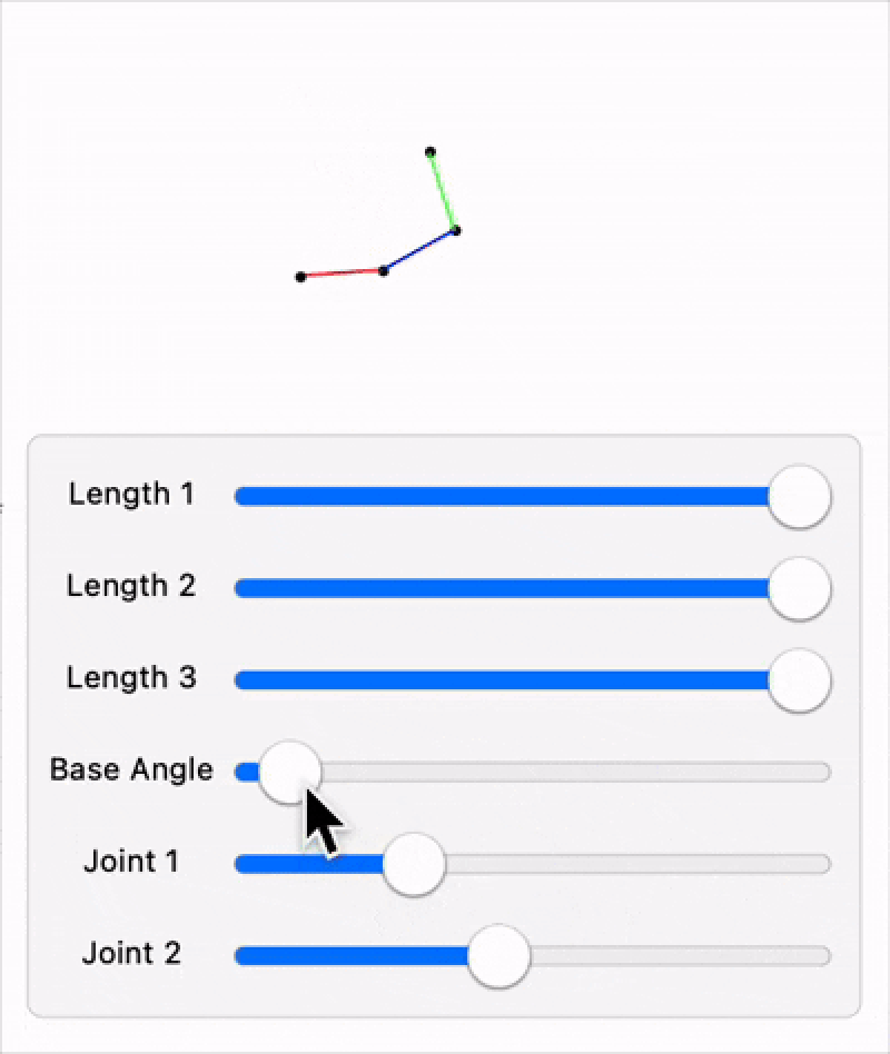
This implementation combines three key Wolfram Language features:
◼
DynamicModule: stores the manipulator’s parameters and preserves their values during interaction.
◼
Graphics: renders the manipulator using geometric shapes such as rectangles and disks to represent links and joints.
◼
Dynamic: automatically changes the graphical representation whenever a specific parameter changes, eliminating the need for redrawing operations.
Exploring the Reachable Workspace
Exploring the Reachable Workspace
Having established the forward kinematic model, the next step is to investigate the range of positions that the manipulator can theoretically reach under different joint angle constraints. Rather than analyzing a single arm configuration, the joint angles are varying continuously through specified angle intervals and the resulting end effector positions were generated using ParametricPlot.
A simplified two-link planar manipulator is used. Although the completely developed robotic arm incorporates three links, reducing the model to two links for workspace generation helps provide clearer visualizations while preserving the same geometric principles for forward kinematics.
Through ParametricPlot, varying the joint angles produces a region representing every position accessible to the manipulator. This representation of this region is known as the reachable workspace. The orange line represents the positions of Joint 1, while the green line and region represent the positions of the end effector (Joint 2).
Three different angular constraints are investigated to examine how limiting the joint rotations influences the overall workspace:
When both joints are restricted to positive rotations only, the reachable workspace contracts further and Joint 1 becomes confined to the first quadrant. While, the end effector can still reach a portion of quadrant 4, the manipulator is unable to access any points with negative y-coordinates. This case demonstrates how directional constraints significantly reduce the attainable end effector positions, even though the manipulator’s physical geometry is unchanged.
For the final configuration, both joints are limited to negative rotations. Joint 1 can now only reach positions below the horizontal axis, while access to the upper half of the plane is limited to a small portion of quadrant 4 for the end effector. This highlights how the orientation of the reachable workspace is heavily influenced by permissible joint rotations where even small changes can limit accessibility.
Time Dependent Motion of The Manipulator
Time Dependent Motion of The Manipulator
After validating the static forward kinematic model, the manipulator was extended to simulate continuous motion by allowing each joint angle to vary as a sinusoidal function of time. Rather than assigning fixed joint angles, the angular position of every joint is represented by a time dependent function,
allowing the manipulator to move continuously while preserving the geometric parameters established by the forward kinematic equations.
The position of each joint is recalculated at every instant using the cumulative joint rotations derived previously. Instead of manually evaluating the trigonometric equations for every frame, this implementation employs the Wolfram Language function RotationTransform, which constructs a rotation matrix for a specified angle and applies it for the corresponding link vector. The endpoint of each link is then obtained by adding the rotated vector to the coordinates of the previous point.
Consequently,
Consequently,
To demonstrate the animation, the joint angles were assigned sinusoidal functions of time,
The animation is implemented using Manipulate, which continuously updates the parameter “t”. At each frame, the joint positions are recomputed and the manipulator is redrawn, producing a real-time simulation of the robotic arm’s motion.
Joint and Angle Definitions
Three-Link Manipulator Setup with Time Assigned
Animated Three-Link Robotic Manipulator
Unlike the earlier implementation, which explicitly evaluates trigonometric expressions for each joint, this version employs RotationTransform to perform the geometric rotations directly. This, therefore, acts as a concise implementation while remaining mathematically equivalent to the forward kinematic formulae approach.
Developing an Intuition for Inverse Kinematics
Developing an Intuition for Inverse Kinematics
Before implementing the complete FABRIK algorithm, it is helpful to understand the fundamental idea behind inverse kinematics using a simple example. Unlike forward kinematics, where the joint angles are known and the end effector is calculated directly, inverse kinematics begins with a desired target position and seeks a joint configuration (typically rotation of the angles) that allows the manipulator to reach that point.
To illustrate this process, a simple three-link manipulator is presented in a fully extended horizontal configuration, while a target point is placed at coordinates (3,4). The objective is to reposition the manipulator so that its end effector converges towards the target while maintaining the fixed lengths of all links.
To illustrate this process, a simple three-link manipulator is presented in a fully extended horizontal configuration, while a target point is placed at coordinates (3,4). The objective is to reposition the manipulator so that its end effector converges towards the target while maintaining the fixed lengths of all links.
Defined Points, Lengths, and Target
Initial Configuration of The Manipulator and Target Position
Rather than immediately solving the entire inverse kinematics problem, the end effector is first moved directly to the target position. This does not yet produce a valid manipulator configuration, as the distance between the prescribed points is no longer equal to the prescribed length. Therefore, the remaining joints must be repositioned while preserving the geometry of the manipulator.
End Effector Moving Directly to Target
A direction vector is first constructed from the end effector towards the previous joint,
which indicates the direction in which the joint must be repositioned. Since only the direction of this vector is required, it is normalized using the Normalize function to produced a unit vector.
The previous joint is then repositioned exactly one link length away from the end effector according to:
The same procedure is repeated for each remaining joint until the base is reached, completing the backward pass.
The forward pass follows the same geometric principle as the backward pass but proceeds in the opposite direction. After the backward pass, the base of the manipulator is no longer fixed at its original location. The forward pass therefore begins by restoring the base to its initial position and then successively repositions each joint while preserving the prescribed lengths. At every step, a direction vector is computed, normalized to obtain a unit vector, and scaled by the corresponding link length before determining the new joint position. This process is repeated until the end effector is reached, completing one full iteration of the FABRIK algorithm.
FABRIK Algorithm
FABRIK Algorithm
Enforcing Joint-Angle Constraints:
Enforcing Joint-Angle Constraints:
The standard FABRIK algorithm preserves the lengths of the manipulator’s links but does not inherently restrict the range of motion of individual joints. Consequently, the computed configuration may violate the physical limits of a real robotic manipulator. To overcome this limitation, a custom helper function was developed to constrain the orientation of each joint during every iteration.
The function accepts two vectors:
The function accepts two vectors:
◼
The Original Vector: representing the orientation of the preceding link.
◼
The Candidate Vector: representing the newly calculated orientation after the FABRIK update.
The angle between these vectors is first determined using the function VectorAngle. Because the angle between two vectors can be measured in either rotational direction, the complementary angle,
2π - θ
is also evaluated. This allows the FABRIK algorithm to distinguish between clockwise and anti-clockwise rotations when investigating whether the calculated orientation lies within the prescribed angular limits.
The ‘If’ function is used to determine whether the newly computed joint orientation satisfies the prescribed angular constraints before any correction is applied.
If the new orientation violates the joint limits, the original vector is rotated to each permissible boundary using RotationMatrix. Therefore, the boundVectors represent the extreme attainable orientations for the joint.
Finally, the corrected vector is selected by comparing the candidate orientation with boundVectors and choosing the one requiring smallest adjustment.
Helper Function
FABRIK:
FABRIK:
Backwards:
Backwards:
The algorithm begins by creating a local copy of the manipulator’s joint coordinates. This stores the original end effector position while allowing the algorithm to modify the joint positions. The initial base position is stored so that it can later be restored during the forward pass. The end effector is temporarily moved directly to the target position, initiating the backward pass.
A Table loop is used to iterate through the joints in reverse order, beginning with the joint immediately before the end effector and ending at the base. At each iteration, the Euclidean distance between two neighboring joints is calculated and used to determine the direction in which the current joint must be repositioned.
After each joint is repositioned, the helper function is used to verify that the new orientation satisfies the specific joint-angle constraints. If the calculated orientation exceeds the range, the helper function returns the nearest valid orientation before the algorithm proceeds to the next joint. Finally, an additional maximum rotation constraint limits the angular displacement between consecutive iterations, preventing unrealistic changes in the manipulator’s configuration.
Once every joint has been updated, the backward pass is complete.
Once every joint has been updated, the backward pass is complete.
Forwards:
Forwards:
Following the backward pass, the base of the manipulator is no longer located at its original position. The forward pass therefore restores the base and makes the joint corrections back towards the end effector.
This mirrors the structure of the backward pass, but the joints are updated from the base towards the end effector. During each iteration, the distance and direction between neighboring joints are recalculated before the current joint is repositioned so that the link length remains constant. The helper function is again applied to enforce the joint-angle limits, while the maximum rotation constraint ensures that the following configurations remain smooth and realistic.
Together the backward and forward passes contribute one complete iteration of the FABRIK algorithm. Repeating these iterations progressively reduces the Euclidean distance between the end effector and the target until the desired level of accuracy is achieved.
Together the backward and forward passes contribute one complete iteration of the FABRIK algorithm. Repeating these iterations progressively reduces the Euclidean distance between the end effector and the target until the desired level of accuracy is achieved.
A Fixed Target Position
A Module is constructed to automate the Inverse Kinematics Simulation. For each trial, random joints coordinates are generated.
Visualizing the sequence of manipulator configurations using ListAnimate.
The animation demonstrates the iterative nature of the FABRIK algorithm. Beginning from a random initial configuration, repeated backward and forward passes gradually reposition the manipulator while preserving its link lengths and satisfying the prescribed joint constraints. As the iterations progress, the Euclidean error decreases until the end effector converges to the target within the specified tolerance.
Experimental Investigation
Experimental Investigation
To evaluate the performance of the inverse kinematics algorithm under a wide range of manipulator configurations, large-scale experimentation was conducted. Rather than analyzing a single manipulator, the algorithm was executed repeatedly using randomly generated link configurations. This enabled the influence of varying link lengths on the convergence behavior and positioning accuracy of the end effector to be investigated statistically.
For each simulation, the FABRIK algorithm was iterated until convergence, after which the final end-effector position, Euclidean error, and corresponding link lengths were recorded. Repeating this process hundreds of times produced a dataset suitable for analysis.
For each simulation, the FABRIK algorithm was iterated until convergence, after which the final end-effector position, Euclidean error, and corresponding link lengths were recorded. Repeating this process hundreds of times produced a dataset suitable for analysis.
Generating Five Hundred Independent Simulations
Organizing the simulation results into a dataset enables the convergence behavior of the algorithm to be examined systematically. Recording both the geometric parameters and the corresponding positioning error allows relationships between manipulator geometry and inverse kinematics performance to be investigated quantitatively.
Since the final frame represents the converged manipulator configuration, only the final iteration from each simulation was extracted. This ensures that all subsequent analyses compare fully converged solutions rather than intermediate iterations.
Selecting the last frame from each Simulation.
A continuous color map is applied to represent the magnitude of the final positioning error, allowing regions of high and low convergence accuracy to be distinguished visually.
The final link lengths from each simulation were visualized using a three-dimensional scatter plot. Each point represents one converged manipulator configuration, where the three axes correspond to the lengths of the individual links. By coloring the points according to their final Euclidean error, it becomes possible to investigate whether particular geometric configurations consistently produce higher or lower positioning errors.
Unlike analyzing individual simulations, this representation reveals broader trends across the entire population of manipulators, allowing the influence of link geometry on inverse kinematics performance to be explored visually.
Unlike analyzing individual simulations, this representation reveals broader trends across the entire population of manipulators, allowing the influence of link geometry on inverse kinematics performance to be explored visually.
To investigate the overall accuracy of the inverse kinematics algorithm, the final Euclidean errors from all simulations were represented using a histogram. Unlike the previous scatter plot, which examines how geometry influences performance, the histogram summarizes the distribution of convergence errors across the entire experimental dataset. A narrow distribution concentrated near zero indicates that the algorithm consistently converges to the desired target regardless of the manipulator’s geometry, whereas a wider distribution would suggest that certain link configurations are more difficult to solve accurately.
The experimental results demonstrate that the FABRIK algorithm converges reliably across a broad range of randomly generated manipulator geometries. While varying the link lengths alters the overall geometry of the manipulator, no strong relationship between individual link lengths and final positioning error was observed. Instead, the algorithm consistently reduced the Euclidean error to values approaching zero, indicating robust convergence under the imposed joint-angle and rotational constraints.
Conclusion
Conclusion
This investigation explored the application of forward and inverse kinematics to a planar three-link robotic manipulator implemented entirely in the Wolfram Language. Beginning with the derivation of the forward kinematic equations, an interactive model was developed to visualize the influence of joint angles and link lengths on the manipulator’s configuration. The implementation was then extended using the Forward and Backward Reaching Inverse Kinematics (FABRIK) algorithm, enabling the manipulator to iteratively reach arbitrary target positions while preserving fixed link lengths and satisfying joint-angle constraints. To evaluate the performance of the algorithm, hundreds of simulations were conducted using randomly generated manipulator configurations. By analyzing the final positioning errors and corresponding link lengths, the investigation demonstrated that the constrained FABRIK implementation converged reliably across a wide range of geometries.
Future Directions
Future Directions
Although the present investigation considers a planar three-link manipulator, several extensions could further enhance the model. One natural progression would be to generalize the implementation to manipulators with a random number of links, allowing more complex robotic systems to be investigated. The algorithm could also be extended to three-dimensional manipulators by incorporating additional rotational degrees of freedom.
Another promising direction would be to investigate optimization techniques for automatically determining link-length configurations that minimize convergence time or maximize the reachable workspace for specific tasks. Additional constraints, including obstacle avoidance, collision detection, actuator limitations, and joint velocity limits, could also be incorporated to more closely model real-world robotic manipulators.
Finally, the implementation could be integrated with physical robotic hardware or simulated environments, allowing the computational model developed in this investigation to be validated experimentally.
Acknowledgements
Acknowledgements
I would like to sincerely thank my mentor, Adam Miller, for his expert guidance, insightful feedback, and continuous support throughout this project. I am especially grateful to Aanya Gupta for her invaluable guidance in understanding and implementing the FABRIK algorithm, and to William Choi Kim for his assistance in overcoming technical challenges encountered during the project. I would also like to thank my advocate Dan McDonald, who’s guidance helped inspire this project. The teaching assistants, Arnay Garyhan and Bryan Chen, for their consistent encouragement and technical support. My thanks also extend to all the other teaching assistants and my mentor group, Samarth Bhar, Akilan Pandian, and Saanvi Raghavendaran whose enthusiasm and support made this experience both enjoyable and rewarding. Thank you to the program directors, Rory Foulger, Megan Davis, Eryn Gillam, Cyrus Taylor for creating a challenging yet exciting research environment, and to Stephen Wolfram for helping brainstorm and shape the initial idea for inspiring this work. Lastly, I would like to thank my parents for providing me this incredible opportunity for which I’m eternally grateful.
References
References
1) Wolfram Research. Wolfram Language & System Documentation Center. Version 14.x. Champaign, IL, USA.
2) Aristidou, A., & Lasenby, J. (2011). https://www.sciencedirect.com/science/article/abs/pii/S1524070311000178 FABRIK: A fast, iterative solver for the inverse kinematics problem. Graphical Models, 73(5), 243–260.
3) Craig, J. J. (2018). Introduction to Robotics: Mechanics and Control (4th ed.). Pearson.
4) EgoMoose. (n.d.). FABRIK (Inverse Kinematics) [Video]. YouTube. https://www.youtube.com/watch?v=UNoX65PRehA
5) Gupta, A. (2025). [WSRP25] Modeling Kathak dancers’ lower bodies through forward and inverse kinematics. Wolfram Community. https://community.wolfram.com/groups/-/m/t/3498889
6) Corke, P. (2017). Robotics, Vision and Control (2nd ed.). Springer
CITE THIS NOTEBOOK
CITE THIS NOTEBOOK
Kinematic analysis and link-length optimization of planar robotic manipulators
by Shashank Bhasin
Wolfram Community, STAFF PICKS, July 9, 2026
https://community.wolfram.com/groups/-/m/t/3754018
by Shashank Bhasin
Wolfram Community, STAFF PICKS, July 9, 2026
https://community.wolfram.com/groups/-/m/t/3754018