A 1D Random Walk with Fractal Dimension 2.0

This Demonstration shows a 1D random walk with fractal dimension 2 retrieved from a numerical experiment. You can get an intuitive insight into how a fractal function of dimension 2 behaves with varying resolution. These functions are extremely important, as they have been shown to be the geometrical foundation of quantum behavior[1].

Details

This Demonstration illustrates the random walk property

σ(N,ϵ)=ϵ

where

is the dispersion,

is the number of steps, and

is the size of a step. The relation

a constant, is here shown to be the signature of a fractal dimension equal to 2.

The fractal dimension of an object is the power that links the number

of smaller objects used to measure it and their typical length

, which is called the resolution.

When

N(ϵ)

is known, then the fractal dimension

is by definition

N(ϵ)

)

, where

is an arbitrary resolution of reference. It can be written

N(ϵ)

=c'

(the constant

is fixed by the arbitrary chosen reference

). The object of reference might be chosen to be the whole main object itself, so that

)=1

, and the definition becomes

N(ϵ)=

Once this law is known, any dimensional measure of the object can be computed: length in

, surface in

, volume in

, "Koch-measure" in

1.26

, or any

measure in

, where

is a dimension of reference (the fractal dimension of the measuring object). In general, the

measure is only finite when

; it tends to 0 when

and to

∞

when

(e.g., a Koch curve has infinite length, null surface, and constant "Koch-measure" measured in

1.26

). The general law is given by

(ϵ)=

(

)

, where

is the

measure. As

ϵ0

, it is clear that the sign of

gives the limit of the

measure (0, constant, or infinite). In other words, at infinite resolution, an object has a finite, non-null measure only when measured in its own (fractal) dimension.

In the case of the usual self-similar fractals, the relation

N(ϵ)

is given recursively by the generator of the fractal, for instance

=4N(ϵ)

for the Koch curve, which, once paired with the definition of

N(ϵ)=

, gives

and hence

log(4)

log(3)

=1.26

But the case of a random walk is different because it is a nondeterministic process, so there is no generator and the curve is not even unique. Nevertheless, it is possible to get the needed relation

N(ϵ)

by statistical means: it is the very definition of the dispersion

σ(N,ϵ)=ϵ

. It then becomes possible to get the dimension of a random curve statistically. The hidden order lies in the rules used to generate the walk: equal probability for each direction and independence of each trial (Markov process).

Here, the needed relation is obtained by imposing that

σ(N,ϵ)

is constant, which amounts to fixing a reference object

σ(1,

)

, for example, the distance between two fixed points. This is consistent with the meaning of the dispersion

σ(N,ϵ)

, which is the mean departure away from the mean value (here

μ=0

) and can be thought of as the mean displacement of the drunken sailor. That

is constant can now be understood as the signature of a fractal dimension 2.

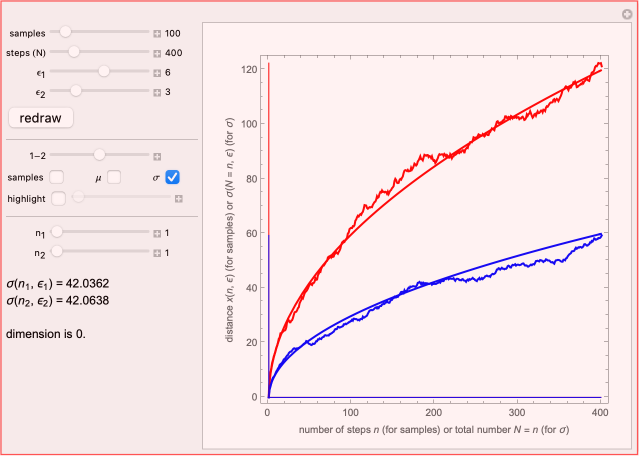
In this Demonstration, two sets of random walks with two different resolutions (step sizes)

and

are computed with their statistical properties

and

You can choose the number of samples, the number

of steps, and the two resolutions

and

. The "redraw" button recomputes new samples with the new chosen values. You can display all the samples (large numbers of samples or steps may be slow on some computers), the mean functions

(with their theoretical value:

μ(N,ϵ)=0

), and the

functions (with their theoretical values:

σ(N,ϵ)=ϵ

The 1-2 slider lets you choose to look at only one set or both and the "highlight" checkbox highlights one sample that you can select with the corresponding slider (this may help to compare individual samples with different resolutions).

When adjusting the sliders

and

so that

σ(

)=σ(

)

, you can check that the computed dimension

log(

)

log(

)

is around 2, with an error depending on how far the experimental

's are from their theoretical values (the more samples, the smaller the error).

The intuitive meaning of all this is that when you compare two random walks at two different resolutions (between two fixed points, here

and

σ(n,ϵ)

), each step contains (on average)

steps

times smaller. You need four small steps to make one step two times larger, nine small steps to make one step three times larger, and so on. Another way to see it is to consider the displacement

as a new step of size

, which contains

steps

, but is only

times larger.

If the fractal dimension of the random walk is unknown from theory, this Demonstration lets you retrieve it by numerical experiment.

Understanding fractal dimensions and fractal functions is particularly important in the light of Laurent Nottale's scale relativity[1], where the spacetime coordinates are functions of their resolutions (and hence are fractal curves). The dimension 2 is especially important, as it has been shown (first by Feynman[2]) that each (fractal) spacetime coordinate acquires dimension 2 at the quantum scale.

References

[1] L. Nottale, Scale Relativity and Fractal Space-Time, London: Imperial College Press, 2011.

[2] R. Feynman and A. Hibbs, Quantum Mechanics and Path Integrals, New York: McGraw–Hill, 1965.

Permanent Citation

Cedric Voisin

"A 1D Random Walk with Fractal Dimension 2.0" from the Wolfram Demonstrations Project http://demonstrations.wolfram.com/A1DRandomWalkWithFractalDimension20/
Published: July 2, 2012