Approximate analytical solutions of the Schrödinger equation for the Eckart-type potential for arbitrary angular momentum
Approximate analytical solutions of the Schrödinger equation for the Eckart-type potential for arbitrary angular momentum
Paul Abbott
School of Physics, Mathematics and Computing
The University of Western Australia
paul.c.abbott@uwa.edu.au
The University of Western Australia
paul.c.abbott@uwa.edu.au
Abstract
A number of recent papers [1-6] consider the time-independent radial Schrödinger equation, for the “Eckart-type” potential
V(r)-α+β,
-r/b
1-
-r/b
-r/b
2
(1-)
-r/b
(
1
)where , for arbitrary angular momentum value . This paper proposes a better approximation for the centrifugal term, , yielding results consistent with numerical methods.
α,β>0
l
l(l+1)/
2
r
I have used Mathematica for the following derivations so that all results can be verified directly.
The Eckart Potential
The Eckart Potential
First, a historical note. In 1930 Eckart [
0
] defined the one-dimensional potentialV(x)A+B,
kx
1+
kx
kx
2
(1+)
kx
(
2
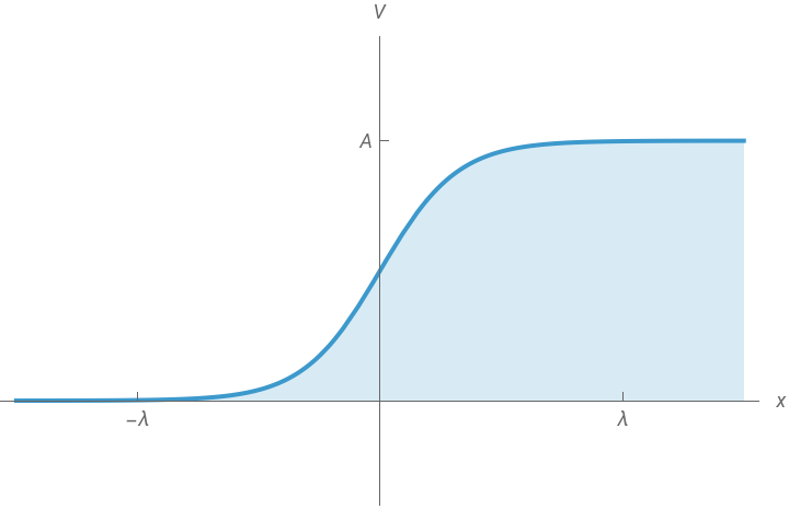
)where , to investigate the tunnelling through a smooth potential barrier. Here λ is the length scale over which the potential is varying.
k=2π/λ


▲
Plots of the Eckart potential ( varies from to .
2
) as the ratio B/A
-3
3
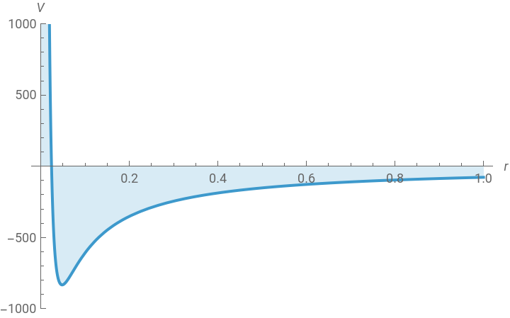
Qualitatively, this is very different to the “Eckart-type” potential (.
2
), which is infinite at r=0
V[α_,β_,b_:1][r_]:=-α+β
-r/b
1-
-r/b
-r/b
2
(1-)
-r/b
▲
Plot of the “Eckart-type” potential for various and .
α1/b
β
Bound-state Solutions
Bound-state Solutions
The paper by Dong et al. [
0
] provides a good introduction to this topic, and a clear—albeit completely standard—treatment of the bound-state solutions. It is worth repeating that treatment here.After factoring off the angular dependence, , the radial Schrödinger equation in atomic units reads
Ψ(r)=R(r)(θ,φ)
m
Y
l
R(r)--2V(r)+2ℰ++(r)0
l(l+1)
2
r
2(r)
′
R
r
′′
R
Putting the equation for reads
R(r)=u(r)
-1
r
u
u(r)--1++-4ℰ-2(r)0
4α
r
b
4β
r
b
2
-1
r
b
2l(l+1)
2
r
′′
u
which is equivalent equation (3) of Dong et al. [ (), energies by , and introducing , , the scaled equation reads
0
]. Scaling lengths by b
rbρ
-2
b
=2α
2
b
ℬ=2β
2
b
u(ρ)2--1++ℬ-4ℰ-2(ρ)0
ρ
l(l+1)
2
ρ
ρ
2
(-1)
ρ
′′
u
No analytic solution is known for this equation when . However, it is easy to obtain approximate solutions by expressing the centrifugal term, , in terms of functions that are “compatible” with the potential.
l≠0
l(l+1)/
2
r
Introducing , the scaled equation reads
z=⟹ρ=-log(z)
-ρ
U(z)-(z)--+2ℰ+(z)+z(z)0
l(l+1)
2
log
z
z-1
zℬ
2
(z-1)
2
z
′′
U
′
U
Expanding the (-dependent part of the) centrifugal term, , into a Taylor series about one obtains,
z
1(z)
2
log
z=1
1
2
(z-1)
1
z-1
1
12
2
(z-1)
Just keeping the first term introduces a Coulomb term [
0
]. The “standard” approximation (see equation (7) of [0
] and [0
]) comprises the first two terms of this series. It is clear from the partial fraction expansion of the “Eckart-type” potential (2
),++
+ℬ
z-1
ℬ
2
(z-1)
that this approximation is “compatible” with the potential in the sense that it is of the same form as the potential itself. Note that the “Eckart-type” potential (,
2
) already has a “Coulomb” component, as is clearly seen by series expansion in ρ
ℬ
2
ρ
ρ
1
12
ρ
12
2
ρ
What is important is the quality of the approximation of the centrifugal or orbital term. The following plot shows the centrifugal term, the “standard” approximation, and the first three terms of the Taylor series, for .
0≤z≤0.35
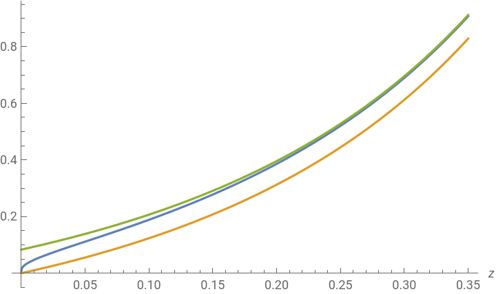


It is clear that taking the first three terms of the Taylor series provides an even better approximation, and that such an approximation is also “compatible” with the potential.
Using the first three terms of the Taylor series, the scaled equation reads
U(z)(-12-l(l+1)+24ℰ)--+(z)+z(z)0
1
12
+l(l+1)+ℬ
z-1
l(l+1)+ℬ
2
(z-1)
2
z
′′
U
′
U
z(1-z)(z)+(c-(a+b+1)z)(z)-abw(z)0
′′
w
′
w
(
3
)has three regular singular points . Putting , the approximate scaled equation reads
z=0,1,∞
U(z)w(z)
κ
z
δ+1
(1-z)
w(z)(12-12-24δκ-24δ-12-24κ+l(l+1)-24ℰ-12)+++(z-)(z)+(z)(2κ-z(2δ+2κ+3)+1)0
1
12
2
δ
2
κ
--δ+l(l+1)+ℬ
2
δ
z-1
12-l(l+1)+24ℰ
2
κ
12z
2
z
′′
w
′
w
To get this in the form of (-2ℰ and +l+ℬ-δ. The physical solution to this quadratic in is
3
), we put 2
κ
l(l+1)
12
2
δ
2
l
δ
δ+4ℬ-1
1
2
2
(2l+1)
Solution of the resulting hypergeometric differential equation,
w(z)(-2δκ-δ-2κ-l(l+1)-ℬ-1)+(z)(2κ-z(2δ+2κ+3)+1)-(z-1)z(z)0
′
w
′′
w
is immediate. However, introducing , simplifies the differential equation to
μ
δ(δ+1)++-ℬ-l(l+1)
-(δ+1)2
κ
′
w
′′
w
and its solution, w(z), then reads
κ
z
c
2
-κ
z
2
F
1
c
1
κ
z
2
F
1
Here and are arbitrary constants. It is clear that these two solutions are related by the interchange and ↔. However, the solution involving is singular at for . The leading term in the series expansion of the other solution (κ-μ,2δ+κ+μ+2;2κ+1;z) about ,
c
1
c
2
κ↔-κ
c
1
c
2
-κ
z
z=0
κ≠0
κ
z
δ+1
(1-z)
2
F
1
z=1
πcsc(2πδ)Γ(2κ+1)
δ
(1-z)
Γ(2δ+2)Γ(κ+μ+1)Γ(-2δ+κ-μ-1)
is proportional to Γ(κ-μ), which is singular unless for . Hence the unnormalized general solution is
-δ
(1-z)
κ-μ-ν
ν∈
0+
U(z)
δ+1
(1-z)
κ
z
2
F
1
where , , and
δ=+4ℬ-1
1
2
2
(2l+1)
ℰ=-
l(l+1)
24
2
κ
2
κ-
-+2δν+δ++l++ℬ
2
l
2
(ν+1)
2(δ+ν+1)
Putting , the energy as a function of the quantum numbers and the potential parameters and reads
ν=n-l-1
ℰ
n,l
(n,l)
=2α
2
b
ℬ=2β
2
b
1
24
2
-++(-l+n-1)+4ℬ-1+++4ℬ-1+l+ℬ
2
l
2
(2l+1)
2
(l-n)
1
2
2
(2l+1)
8
2
+4ℬ-1-l+n
1
2
2
(2l+1)
Rewriting this in terms of the potential parameters , , and the scale parameter , one has
α
β
b
ℰ
n_,l_
1
2
b
ℰ
n,l
2
b
2
b
The case — the Hulthén potential — reduces to
β=0
l(l+1)
24
2
b
2
(-2α)
2
n
2
b
8
2
b
2
n
Variational Energies
Variational Energies
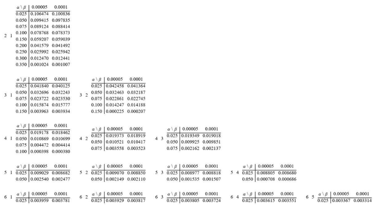
To assess the quality of these results, it is straightforward to compute accurate energy eigenvalues using standard variational methods. Using integration by parts, the radial Schrödinger equation can be rewritten as
where the required matrix elements can be computed directly as numerical integrals,
Introducing the matrix element,
and using hydrogenic radial wave functions,
Pre-requisites
Pre-requisites
Now, we can directly manipulate equations.
References
References