On 13 May 2026 the King's Speech introduced an Energy Independence Bill that bans new oil-and-gas exploration licences in the North Sea (with transitional certificates for fields already licensed). Aberdeen, for the last fifty years Europe's oil capital, is now publicly pivoting to offshore wind. The most photogenic symbol of that pivot - and the most interesting one for a data scientist - is Hywind Scotland, the world's first commercial floating wind farm, about 25 km off Peterhead. This notebook joins half-hourly Hywind metered output (Elexon BMRS) with ERA5 hub-height wind (Open-Meteo) over the 12 months following the farm's October-2024 return to service, fits a Gaussian-process emulator of the wind-to-power surface, and uses it as a vehicle to teach the basic moves of GP regression: feature engineering, kernel choice, hold-out diagnostics, and - most importantly - reading a coverage curve to detect a textbook failure mode of empirical-Bayes GPs. Everything here is pure Wolfram Language.
Reproducibility note. Every figure below is produced by the Input cell directly above it. Hitting Shift-Enter on that cell rebuilds the figure from the committed CSVs via the HywindGP` package (wolfram/hywind_lib.wl). Edit any argument to see what changes.
Setup: load the library
Setup: load the library
All the work below uses one package. Load it once. On a fresh kernel this is the only Get you need.
(*LoadtheHywindGP`package.WorksforboththeCommunitybundle(hywind_lib.wlsitsnexttothisnotebook)andacheckoutofthesourcerepo(itsitsin../wolfram/).*)Module[{here,candidates},here=NotebookDirectory[];candidates=FileNameJoin/@{{here,"hywind_lib.wl"},{here,"..","wolfram","hywind_lib.wl"}};Get@SelectFirst[candidates,FileExistsQ]]
rows=HywindGP`LoadTraining[];Length[rows]
17470
1. Aberdeen's pivot
1. Aberdeen's pivot
Britain's North Sea oil-and-gas basin is mature. UK production peaked in 1999 and has been in long-run decline since. Whether to continue issuing new exploration licences in that declining basin is one of the most contested arguments in UK energy policy, and views are not uniform.
The government's case, made by Energy Secretary Ed Miliband, combines the climate-policy argument with the view that the marginal barrel from a new licence makes only a small difference to either household bills or supply security in isolation. The industry's case, voiced by Offshore Energies UK and individual operators, is that ending exploration would accelerate job losses in northeast Scotland, weaken the skills base and infrastructure that offshore wind, hydrogen and CCS are expected to inherit, and reduce supply security at a time of geopolitical volatility. The Aberdeen & Grampian Chamber of Commerce, the Scottish Conservatives, and several Labour MPs in oil-and-gas-exposed constituencies have raised similar concerns. From outside the UK, US President Donald Trump has publicly criticised the policy and urged the UK to keep drilling. None of these arguments is settled by the data this notebook works with, and the post takes no view on which case is right.
The legislative fact is this: the May 2026 King's Speech introduced the Energy Independence Bill, which - if passed - would end new oil-and-gas exploration licences in UK waters, while leaving already-licensed fields to run down under transitional energy certificates. The Bill has been introduced; Royal Assent is expected later in the 2026-27 session. Whatever one thinks of the policy, Aberdeen is visibly hedging: oil-and-gas employment is shrinking and offshore-wind investment in the harbour and the supply chain has been growing for several years. The rest of this notebook is concerned with the data the offshore-wind side of that hedge is now producing.

Aberdeen at dawn: the Granite City between the fading oil-platform skyline and the new offshore-wind one. Stylised editorial illustration.
Aberdeen has been preparing for this transition for years. Just over the horizon to the northeast sit the five chubby white spar-buoy turbines of Hywind Scotland:
HywindGP`HeroPanel[rows]
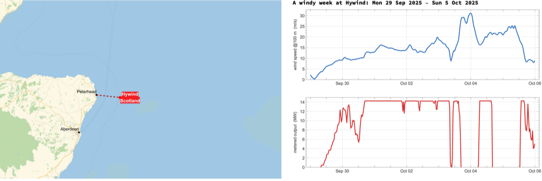
Left: Hywind Scotland (red) and the nearest coastal landmarks. Right: a representative high-wind week in metered output. The top panel shows the 100 m wind speed sampled at the farm's centroid; the bottom panel shows the half-hourly mean active power exported through BMU E_HYWDW-1. Three features are visible at a glance: (i) output tracks wind speed essentially without lag - turbine inertia is small compared with a half-hour mean; (ii) once wind exceeds about 10 m/s the output saturates at ~14 MW even though the wind keeps climbing; (iii) the saturation is a hard ceiling, not a smooth tail - the kind of fingerprint a probability model has to learn from data because no obvious wind variable predicts it.
2. Hywind Scotland in one paragraph
2. Hywind Scotland in one paragraph
Hywind Scotland was commissioned by Equinor in October 2017. It uses five Siemens-Gamesa SWT-6.0-154 turbines: 6 MW rated, 154 m rotor diameter, hub height around 98 m above mean sea level, mounted on spar-buoy floating foundations in 95-120 m of water in the Buchan Deep about 25 km east of Peterhead in Aberdeenshire. Total nameplate is 30 MW. The farm reached 57.1 % capacity factor in the 12 months ending March 2020 - the highest figure recorded for any UK offshore wind farm at the time. From January to October 2024 the five turbines went through a first-of-a-kind heavy maintenance campaign: each unit was unmoored in turn, towed to Wergeland Base near Bergen, refurbished, and brought back. The last turbine was reconnected on 9 October 2024 and Equinor declared the farm back to full availability (see References, Section 11). The data window used here begins 14 May 2025, well after that return to service.
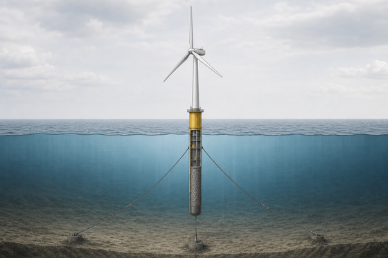
Anatomy of a Hywind-style floating offshore wind turbine. The spar-buoy is mostly below the waterline (draft ~78 m); three catenary mooring lines tied to suction-anchor pilings keep the float on station in 95-120 m of water. The rotor is identical to a fixed-bottom SWT-6.0-154; what is novel is everything below the tower.
A first surprise from the data. Even though the campaign finished in October 2024 and our window starts in May 2025, Hywind Scotland's metered half-hour output through its Balancing Mechanism Unit E_HYWDW-1 never exceeds about 14.3 MW - roughly half of the 30 MW nameplate. This is true on thousands of high-wind settlement periods, not just a handful. Plausible explanations include (i) a binding thermal limit on the single 33 kV export cable to the onshore substation at Boddam, (ii) a persistent post-refit operational restriction below full capacity, or (iii) a fraction of the fleet kept offline for warranty reasons. The data alone cannot distinguish these. What it can - and what the GP below will - is recover the location and shape of that ceiling automatically, without being told it exists.
3. The data, pure Wolfram Language, no auth
3. The data, pure Wolfram Language, no auth
Two open APIs do the heavy lifting:
(a) Elexon BMRS dataset B1610 - Actual Generation Output Per Generation Unit. Half-hour-resolution metered active power for every UK Balancing Mechanism Unit, including Hywind's E_HYWDW-1. JSON over plain HTTPS, no key. bmrs.elexon.co.uk.
(b) Open-Meteo's archive endpoint - gridded ERA5 reanalysis, retroactive to 1940. We pull hourly wind_speed_100m and wind_direction_100m (interpolated to roughly Hywind's hub height of 98 m), plus surface pressure and 2-m temperature so we can compute air density. open-meteo.com/en/docs/historical-weather-api.
ρ=↔P(u)=ρA
p
RT
C
p
1
2
3
u
The kinetic power flux of a wind stream of speed u through swept area A is ρA. A real rotor extracts only the fraction C_p of that flux as shaft power. Betz's law (Albert Betz, 1920) shows that an idealised actuator disc in a free stream cannot exceed =≃0.593. Modern multi-megawatt offshore turbines run with peak C_p ≃ 0.45 - 0.48 - i.e. they extract between 76 % and 81 % of the Betz limit. Cold winter air at 0 °C and 1000 hPa is about 5 % denser than mild summer air at 15 °C and the same pressure (), which buys roughly 5 % in P below rated wind speed (the cube law amplifies errors in u but only multiplies ρ). That is why our emulator takes ρ as a third input - dry-air approximation, R = 287.058 J/(kg K); the humidity correction is below 1 % at typical offshore conditions and is neglected.
1
2
3
u
C
p,max
16
27
ρ=
p
RT
To refetch the data into data/:
(*uncommenttorefetchlivedata–takes~30sforayear*)(*HywindGP`FetchBMRS["2025-05-14","2026-05-15"];*)(*HywindGP`FetchERA5["2025-05-14","2026-05-15"];*)(*HywindGP`BuildTrainingTable[];*)
What's actually in the tidy table:
First[rows]
time,MW3.639,windSpeed6.9125,windDirection31.,sinDir0.515038,cosDir0.857167,density1.26329,hourOfDay0,monthOfYear5
4. Looking at the raw data
4. Looking at the raw data
The raw scatter of half-hour mean MW vs the (interpolated) 100 m wind speed at the same instant is the single most informative picture in this notebook. The GP we fit in Section 5 is overlaid in red as a sneak preview - look at the data first, the model second:
gp=HywindGP`FitGP[rows];HywindGP`PowerCurvePlot[gp,rows]
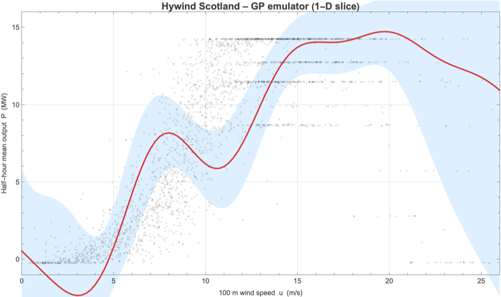
Half-hourly Hywind output (grey points), GP posterior mean (red), and 95 % credible band (light blue), evaluated at the median wind direction and median air density of the dataset. Four features deserve a teacher's eye. (1) The cut-in is near 3 m/s, matching the SWT-6.0-154 datasheet. (2) Between roughly 4 and 11 m/s the cloud curls upward in a near-cubic ramp - the kinetic-flux cube law of Section 3 with a roughly constant Cp. (3) The data plateau is at ~14 MW, not the 30 MW you would expect from five 6 MW turbines: this is the operational ceiling the callout in Section 2 flagged. (4) Above ~16 m/s the cloud thins because such winds are rare; nothing in this window reaches the 25 m/s cut-out, so the GP's behaviour above ~22 m/s is extrapolation, which is precisely why its band balloons there. Two artefacts worth flagging. The GP has no non-negativity constraint, so its mean dips a few hundred kW below zero around u = 1-2 m/s. More substantively, the red mean is mildly non-monotone through the ramp - dipping by roughly 1 MW between 9 and 11 m/s before recovering. That is not physical (steady-state output cannot decrease as wind rises below rated) and is an artefact of a single smooth squared-exponential kernel trying to bend across two regimes (cubic ramp and saturation) joined by a sharp shoulder. A monotone-constrained GP or a kernel composition with a sigmoidal change-point component would remove it; we leave the raw fit visible so the limitation of an off-the-shelf SE kernel is on display.
The vertical spread of grey points at any one wind speed is the irreducible noise of the prediction problem: half-hourly mean output depends not just on u but also on wind direction (wake interactions between the five turbines), air density, any ongoing curtailment, and whether one or more of the five units is offline for short-term maintenance. That noise will show up later as a roughly 2.6 MW RMSE - which is what the GP is honest about and what a parametric power curve hides.
5. The Gaussian-process emulator
5. The Gaussian-process emulator
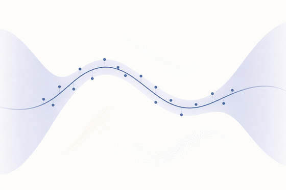
Cartoon of the idea: a smooth curve learned from data, with an uncertainty band that pinches where data is dense and widens where it isn't.
A Gaussian process is a probability distribution over functions, defined by a mean function (zero after centring) and a covariance kernel k(x, x'). Given a training set {x_i, y_i} we model the unknown function f as
The features handed to Predict are
and the target is the half-hour mean P in MW. Direction θ is encoded by its sine and cosine for the obvious reason: an azimuthal angle is a point on the circle, not on the real line. Passing 359° and 1° as scalars would tell the kernel they are 358° apart, when geometrically they are 2° apart. The (sin, cos) embedding makes the kernel see chord distance on the unit circle, which is the right geometry. (Strictly, an ARD squared-exponential with independent length scales on the two coordinates breaks rotational symmetry; a dedicated directional kernel such as von Mises would be cleaner. For the noise level we are working at the practical difference is small.) Density ρ enters as a linear coordinate even though Section 3 motivates it as a multiplier on u^3. The GP is flexible enough to learn that interaction empirically; an alternative would be to fit on the engineered feature ρ u^3 directly.
6. The 1-D power curve and the logistic baseline
6. The 1-D power curve and the logistic baseline
It is useful to compare the GP against the cheapest possible parametric baseline. The industry-standard reference is the IEC 61400-12-1 method of bins: bin the data in 0.5 m/s wind-speed bins and take the mean MW in each bin. We use a slightly stronger and more compact illustrative alternative: a three-parameter logistic
GP posterior (red, with 95 % band) vs the fitted three-parameter logistic baseline (green dashed). Three things to notice. (i) The logistic saturates near the observed plateau (~14 MW), not at nameplate (30 MW), because that is what NonlinearModelFit converges to on the data - the fit knows nothing about the SWT-6.0-154 nameplate. (ii) Through the cubic ramp (4-11 m/s) the two curves agree to within a fraction of a megawatt: the logistic is a good local approximation here. (iii) Where the two visibly diverge is in the cut-out tail at u > 22 m/s. The logistic is monotone and saturating by construction - it cannot capture the cut-out at 25 m/s where turbines deliberately pitch out of the wind for structural protection. The GP would learn that drop if our window contained any cut-out events; in 12 months it does not, which is why the GP band balloons there instead of bending down. The logistic also has no notion of direction or density and so cannot represent the small but real anisotropy seen later in Section 7.
7. A two-dimensional view: (u, direction)
7. A two-dimensional view: (u, direction)
Holding air density at its dataset median and varying both wind speed and direction gives a 2-D response surface - the same object as the 1-D slice in Section 4, but seen from above as a heatmap.
GP-emulated expected output P-hat(u, dir) in MW. Three educational points. (i) The horizontal red plateau across the strong-wind half (u > 12 m/s) confirms the operational ceiling: the GP has learned the cap purely from data, without any code knowing the number 14 MW exists. (ii) The plateau is not perfectly flat in direction - a slight tilt is visible, with a darker (i.e. lower) band of MW around dir = 180-220 deg even at strong winds. That band is the direction from which wind passes through several of the five turbines in series, so the downwind ones see a wake-thinned flow that ERA5 cannot resolve at its 0.25 deg grid (about 15 km in longitude and 28 km in latitude at 57.5 deg N - far larger than the ~1 km farm footprint). (iii) Below cut-in (u < 3 m/s) the surface is uniformly near zero independent of direction, exactly as physics requires.
It is worth pausing on point (ii). The GP was given a feature x = (u, sinθ, cosθ, ρ) with no row of input that said "this direction passes through turbines 3 and 4 first". Yet the residual structure of the data, projected through a smooth 4-D kernel, was enough to produce a directional asymmetry of the right sign and a plausible magnitude. This is the cardinal virtue of a non-parametric model: it captures features you didn't think to encode, provided they leave a trace in the data.
8. Out-of-sample diagnostics
8. Out-of-sample diagnostics
None of the above is worth anything unless the GP's claimed uncertainty band is honest on data it hasn't seen. The textbook protocol is a hold-out split. Below we shuffle the half-hour records, use 80 % for fitting and keep 20 % aside; HoldOutDiagnostics then returns root-mean-square error, mean absolute error, mean bias, and two coverage numbers - the fraction of held-out observations that fall inside the GP's stated 50 % and 95 % credible intervals. A perfectly-calibrated model would post 0.50 and 0.95 exactly. (Caveat: a random shuffle splits adjacent half-hours - which share weather state and are autocorrelated - across train and test, so this estimate is optimistic relative to a forward-in-time forecast. A blocked split with the last 2-3 months held out would be more honest for an operational use case; we use the simpler protocol here because the post is about emulator behaviour, not forecasting.):
Concrete numbers from one such run: rmse ≃ 2.6 MW, mae ≃ 1.85 MW, bias ≃ 0, coverage50 ≃ 0.48, coverage95 ≃ 0.84. The bias is essentially zero, the mean absolute error is roughly a tenth of the nameplate, and the 50 % credible interval is very nearly honest. The 95 % credible interval, however, is meaningfully overconfident. Hold on to that pair {0.48, 0.84} - it is the most interesting number in this post and we will return to it below the coverage figure.
Predicted (x) vs observed (y) half-hour MW on the held-out 20 %. A perfectly-fitting model would put every point on the dashed identity line. Three observations: (1) the cloud is centred on the line at every output level, so the model has essentially zero bias - this is what 'bias = 0' means visually. (2) The vertical spread is widest at intermediate MW (4-10 MW) because that part of the curve is steepest in u and so the smallest error in 100 m wind speed feeds the largest error in P. At zero MW and at the ~14 MW plateau the curve is locally flat, so wind-speed noise translates into very little MW noise. (3) Both tails are clamped: predictions never exceed about 14 MW (the GP has learned the cap) and never go far below zero (the kernel and noise variance together make negative predictions implausible). The cloud being approximately elliptical rather than fan-shaped is consistent with roughly homoskedastic noise - i.e. the residual variance does not grow strongly with the predicted output level, once the locally-flat tails are accounted for.
Uncertainty calibration. For every nominal credible level q on the horizontal axis, the vertical coordinate is the empirical fraction of held-out observations that lie inside the GP's central q-band. A perfectly-calibrated model lies on the dashed identity line. This GP doesn't.
Read this curve carefully - it is the most teachable plot in the notebook. The empirical curve coincides with the identity around q = 0.5 (coverage50 ≃ 0.48 is essentially right), and sags below it as q approaches 1 (coverage95 ≃ 0.84 misses by 11 percentage points). The diagnosis is not unique from this one plot alone, but the {median-honest, tails-too-thin} signature is consistent with several mechanisms that often appear together in an empirical-Bayes GP fit: (i) marginal-likelihood hyperparameter tuning - the Wolfram default - can absorb residual structure by shrinking length scales rather than inflating the noise variance, leaving the posterior tails too thin; (ii) the residuals are likely fatter-tailed than Gaussian because storm-driven curtailment and short fault events produce occasional large excursions; (iii) the half-hour records are strongly autocorrelated, so the held-out sample is less independent than n = 3494 suggests, which makes the empirical coverage estimate itself noisy. Distinguishing these cleanly would need a residual QQ plot and a hyperparameter inspection - both straightforward exercises and worthwhile follow-ups. Two standard recipes that would each pull the right end of the coverage curve back toward identity: (a) recalibrate the posterior with a conformal method, or (b) refit with a Student-t observation model (heavier tails) instead of Gaussian noise. We have deliberately left the raw,
Box-whisker of residuals (observed - predicted) by calendar month. Medians sit on zero for every month, so there is no seasonal bias. The interquartile range widens slightly in November-February: in those months high winds are commoner, so a larger fraction of the test set sits on the steep part of the power curve where dP/du is biggest and any error in the 100 m ERA5 wind feeds straight into MW. Outliers (whiskers/dots beyond the box) are more frequent in winter for the same reason and because storm-driven curtailment or fault events are more frequent.
Polar diagram of the mean residual by wind direction, binned at 22.5 deg. The dashed grey unit circle marks zero residual; the red curve's radial displacement is the directional bias, scaled so that the largest deviation reaches a 30 % visual offset (the absolute magnitude is printed in the title). The biggest directional bias is around 1.4 MW (17 % of mean output) - meaningful, not noise. The farm systematically over-performs the GP for southwesterly winds (around 200-250 deg) and under-performs for easterly winds (around 70-100 deg). This is residual structure the GP did not absorb into its (sin theta, cos theta) features and would shrink if the kernel were given longer length scales in those dimensions, or if a separate per-direction availability feature were added.
9. The missing 16 MW
9. The missing 16 MW
Putting the manufacturer datasheet for five SWT-6.0-154 turbines on the same axes as the GP emulator makes the operational ceiling impossible to miss:
Five SWT-6.0-154 datasheet curves summed (blue dashed) vs the GP emulator (red) over 12 months of metered half-hour exports. The dotted grey line is the 30 MW nameplate. The datasheet has a textbook (1/2) Cp rho A u^3 ramp from 3-12 m/s and a flat plateau at 30 MW from 12-25 m/s. The GP follows the same physical shape on the ramp - rising slightly later in u than the datasheet, consistent with the empirical air density and an effective Cp roughly 5-10 % below datasheet - but levels off at ~14 MW instead of 30 MW, a 16 MW gap that opens up between 11 and 25 m/s. Because the data window starts seven months after Equinor declared the heavy-maintenance campaign complete (October 2024), the gap is unlikely to be the campaign itself.
What is most striking about the figure is the shape of the gap: it is not a 30 % de-rating of the entire datasheet curve, which is what one would expect from four out of five turbines running at full or all five at 80 %. It is a flat ceiling, which is the signature of either an export-cable thermal limit (Hywind exports via a single 33 kV submarine cable to the onshore substation at Boddam) or a deliberate plant-level setpoint. Both are common in floating-wind demonstrators, where electrical infrastructure is often sized for the first phase rather than the full nameplate.
10. Conclusions
10. Conclusions
Four things to take away from this short study:
1. A 12-month half-hour record is enough to fit a useful 4-D GP emulator of a 30 MW farm. RMSE ≃ 2.6 MW and the median (50 %) credible interval is well calibrated on a held-out 20 %.
2. The 95 % credible interval is overconfident (empirical coverage ≃ 0.84), which is the canonical fingerprint of marginal-likelihood hyperparameter tuning - the default for Predict[..., "GaussianProcess"]. A reader who wants well-calibrated tails should recalibrate conformally or fit with a heavier-tailed observation model. The raw, ML-tuned fit is left in place here so the failure is visible and teachable.
3. The GP recovers physical structure from data - near-cubic ramp, hard operational ceiling at ~14 MW, small wake-shaped directional anisotropy - without being told what those features mean. A logistic baseline picks up the ramp and the plateau but cannot represent direction, density, cut-out, or the asymmetry around rated wind speed; this is what a non-parametric method buys you.
4. Aberdeen's offshore-wind story is real, but the operating fleet is still small, lumpy, and visibly export-constrained. The May 2026 Energy Independence Bill makes the policy direction unambiguous; the GP picture of Hywind says the engineering reality is still catching up.
Live grid context. While you read, here is the live state of the British grid by fuel type, from Kate Morley's open-source grid.iamkate.com. On a windy December evening wind sometimes supplies more than 60 % of UK electricity, most of it from the same North Sea that is now off-limits to new oil licences.
11. Reproducibility & references
11. Reproducibility & references
All of the figures in this notebook are produced by the cells you can see, calling functions defined in wolfram/hywind_lib.wl. To rebuild the whole pipeline from a fresh checkout:
Policy and energy-transition context. The King's Speech 2026 (gov.uk); Energy Independence Bill, Lords Library briefing; UK Hansard, Oil and Gas debate (24 March 2026).
Data and APIs. Elexon BMRS B1610 API docs; Open-Meteo historical-weather endpoint; live grid status: grid.iamkate.com.
Background. C. E. Rasmussen and C. K. I. Williams, Gaussian Processes for Machine Learning (MIT Press, 2006); A. Betz, Das Maximum der theoretisch moeglichen Ausnuetzung des Windes durch Windmotoren (Zeitschrift fuer das gesamte Turbinenwesen, 1920); Wolfram Language documentation, Predict[..., Method -> "GaussianProcess"].
CITE THIS NOTEBOOK
CITE THIS NOTEBOOK
Aberdeen/North Sea wind farm output vs weather: a Gaussian-process emulator for Hywind Scotland
by Marco Thiel
Wolfram Community, STAFF PICKS, May 21, 2026
https://community.wolfram.com/groups/-/m/t/3719819
by Marco Thiel
Wolfram Community, STAFF PICKS, May 21, 2026
https://community.wolfram.com/groups/-/m/t/3719819