"Correlation is not causation" is one of the most repeated mantras in science and statistics. But if correlation alone cannot establish causal claims, how do we formalize the leap from statistical association to genuine cause-and-effect reasoning?
The answer lies at the intersection of probability theory and graph theory: Bayesian networks. Introduced in the 1980s and brought to full maturity by Judea Pearl (2000) in his landmark Causality: Models, Reasoning, and Inference, and thoroughly systematized by Koller & Friedman (2009) in Probabilistic Graphical Models, Bayesian networks provide a compact and intuitive language for encoding probabilistic dependencies among a set of random variables.
But Bayesian networks are more than just a clever data structure for probabilities. When their edges are given a causal interpretation, they become the foundation for a complete theory of causal reasoning; one that allows us not only to predict what we will see, but also what will happen if we do something, and even what would have happened under different circumstances.
In this article, we will use the Wolfram Language to explore Bayesian networks.
1 What is a Bayesian Network?
1
What is a Bayesian Network?A Bayesian network (also called a belief network or Bayes net) is defined by two components:
1. A Directed Acyclic Graph (DAG): Each node represents a random variable, and each directed edge represents a direct probabilistic dependency. The graph must be acyclic, ie. you cannot follow the arrows and return to where you started.
2. Conditional Probability Tables (CPTs): For each node, a table specifying the probability of each value of that node given every combination of values of its parents in the DAG.
The key insight is the local Markov property: each variable is conditionally independent of all its non-descendants given its parents. This property is what allows the joint distribution to factor into a product of local terms, dramatically reducing the number of parameters needed.
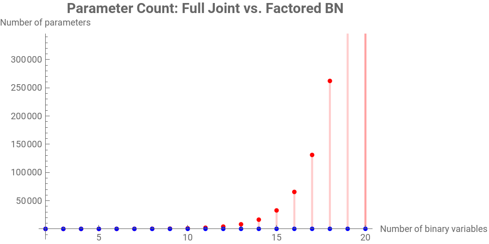
For n binary variables, the full joint distribution requires-1 parameters. A Bayesian network with bounded parent sets can represent the same distribution with far fewer. Let us quantify this advantage.
For n binary variables, the full joint distribution requires
n
2
Out[]=
Parameter Count Comparison | ||||||||
| ||||||||
The savings grow exponentially with the number of variables! |
Exponential growth of full joint vs bounded-parent factored
ShowDiscretePlot2^n-1,{n,2,20},,DiscretePlotn*2^3,{n,2,20},,
Out[]=


2 The Three Fundamental Structures
2
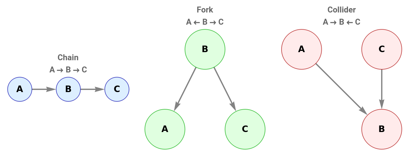
The Three Fundamental StructuresEvery pattern of conditional independence in a Bayesian network can be understood through three fundamental building blocks involving exactly three nodes. Understanding these structures is the key to reading off independence relationships from the graph.
1. Chain (Serial connection): A B C
Information flows from A to C through B. However, if we observe (condition on) B, then A and C become independent. Knowing B blocks the information path. Example: Fire Smoke Alarm. If we know there is smoke, learning about fire tells us nothing new about the alarm.
2. Fork (Diverging connection): A ← B C
B is a common cause of both A and C. Marginally, A and C are dependent (correlated through their shared cause). But conditioning on B renders A and C independent. Example: Temperature ← Season Rainfall. Knowing the season makes temperature and rainfall independent.
B is a common cause of both A and C. Marginally, A and C are dependent (correlated through their shared cause). But conditioning on B renders A and C independent. Example: Temperature ← Season Rainfall. Knowing the season makes temperature and rainfall independent.
3. Collider (Converging connection): A B ← C
B is a common effect of A and C. Marginally, A and C are independent. However, conditioning on B (or any descendant of B) induces a dependence between A and C. This is the famous “explaining away” effect. Example: Talent Admission ← Legacy. Knowing someone was admitted makes talent and legacy status dependent: if they are a legacy admit, they are less likely to be talented.
B is a common effect of A and C. Marginally, A and C are independent. However, conditioning on B (or any descendant of B) induces a dependence between A and C. This is the famous “explaining away” effect. Example: Talent Admission ← Legacy. Knowing someone was admitted makes talent and legacy status dependent: if they are a legacy admit, they are less likely to be talented.
The three fundamental structures as colored graphs
GraphicsRowGraph{"A"->"B","B"->"C"},,Graph{"B"->"A","B"->"C"},,Graph{"A"->"B","C"->"B"},,ImageSize->Full
Out[]=
Summary of information flow rules:
• Chain and Fork: Information flows unless the middle node is observed (conditioning blocks the path).
• Collider: Information is blocked unless the middle node (or a descendant) is observed (conditioning opens the path).
These simple rules, applied systematically, give rise to the powerful concept of d-separation (Section 9).
3 Building Our First Bayesian Network
3
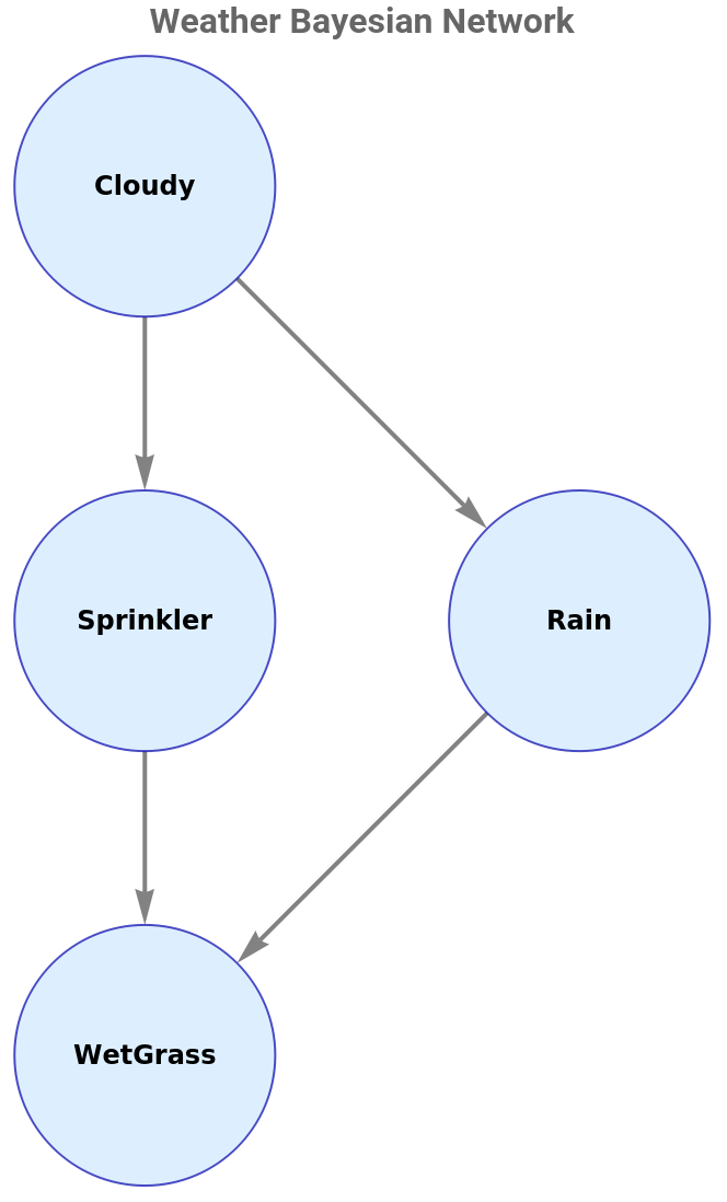
Building Our First Bayesian NetworkLet us build the classic Weather network, a simple but instructive example with four binary variables (each taking values 0 or 1):
• Cloudy : Is it cloudy today? (root node, no parents)
• Sprinkler : Is the garden sprinkler on? (depends on Cloudy)
• Rain : Is it raining? (depends on Cloudy)
• WetGrass : Is the grass wet? (depends on Sprinkler and Rain)
The causal story: on cloudy days, rain is more likely but the sprinkler is less likely to be turned on (you don't water the garden when rain is expected). Both rain and the sprinkler can independently make the grass wet. Notice that the graph captures the direction of causation: clouds cause rain, not the reverse.
weatherDAG=Graph{"Cloudy"->"Sprinkler","Cloudy"->"Rain","Sprinkler"->"WetGrass","Rain"->"WetGrass"},
Out[]=
Verify fundamental graph properties
Column[{Row[{"Is a DAG (acyclic)? ",AcyclicGraphQ[weatherDAG]}],Row[{"Topological order: ",TopologicalSort[weatherDAG]}],Row[{"Number of nodes: ",VertexCount[weatherDAG]}],Row[{"Number of edges: ",EdgeCount[weatherDAG]}],Row[{"Adjacency matrix:"}],MatrixForm[AdjacencyMatrix[weatherDAG]]},Spacings->1]
Out[]=
Is a DAG (acyclic)? True | ||||||||||||||||
Topological order: {Cloudy,Rain,Sprinkler,WetGrass} | ||||||||||||||||
Number of nodes: 4 | ||||||||||||||||
Number of edges: 4 | ||||||||||||||||
Adjacency matrix: | ||||||||||||||||
|
Defining the Conditional Probability Tables
Defining the Conditional Probability Tables
We represent each Conditional Probability Table (CPT) as a nested Association : the outer key is a list of parent values, and the inner key is the node's own value, mapping to a probability.
In[]:=
(*CPTsasnestedAssociations*)(*Format:<|{parentVal1,parentVal2,...}-><|nodeVal->P,...|>|>*)cptCloudy=<|{}-><|0->0.5,1->0.5|>|>;cptSprinkler=<|{0}-><|0->0.5,1->0.5|>,(*sunny:50%chancesprinklerison*){1}-><|0->0.9,1->0.1|>(*cloudy:only10%chancesprinklerison*)|>;cptRain=<|{0}-><|0->0.8,1->0.2|>,(*sunny:20%chanceofrain*){1}-><|0->0.2,1->0.8|>(*cloudy:80%chanceofrain*)|>;cptWetGrass=<|{0,0}-><|0->1.0,1->0.0|>,(*nosprinkler,norain:grassisdry*){0,1}-><|0->0.1,1->0.9|>,(*nosprinkler,rain:90%wet*){1,0}-><|0->0.1,1->0.9|>,(*sprinkler,norain:90%wet*){1,1}-><|0->0.01,1->0.99|>(*both:99%wet*)|>;cpts=<|"Cloudy"->cptCloudy,"Sprinkler"->cptSprinkler,"Rain"->cptRain,"WetGrass"->cptWetGrass|>;
Heatmap visualization of the WetGrass CPT
Helper function and parent structure
Joint probability : product of all local CPT lookups
Generate all 2^4 = 16 possible assignments
Joint distribution must sum to 1
Step - by - step factorization example
Display the full joint distribution as a table
The real power of a Bayesian network lies in answering queries of the form P(Query | Evidence). Given some observations (evidence), what can we infer about unobserved variables?
We implement inference by enumeration: we sum the joint probability over all assignments consistent with the evidence. While this is exponential in the worst case, it is exact and sufficient for small networks like ours.
Two fundamental types of reasoning arise:
• Diagnostic (bottom-up): From effects to causes. "The grass is wet did it rain?"
• Causal (top-down): From causes to effects. "It is cloudy will the grass be wet?"
A Bayesian network handles both directions of reasoning equally well.
Suppose we observe that the grass is wet. What can we infer about rain? About the sprinkler? About cloudiness? This is diagnostic reasoning — we reason backward from observed effects to their likely causes.
Visualize diagnostic reasoning
Conversely, if we know the sky is cloudy, how does this affect the probability of wet grass? And if we then also learn it is NOT raining, what happens?
Observation: Cloudiness increases the probability of wet grass (from about 0.35 to 0.77) because cloudy weather brings more rain. But if we additionally learn it is NOT raining despite the clouds, the probability drops sharply; the sprinkler alone (which is unlikely on cloudy days) must account for any wetness.
One of the most striking and counterintuitive results in Bayesian networks is explaining away (also known as Berkson's paradox or inter-causal reasoning).
In our weather network, Rain and Sprinkler are marginally independent given Cloudy. But if we observe their common effect WetGrass=1, they become dependent. Learning that it rained "explains away" the wet grass, making the sprinkler less likely.
This cannot happen in purely correlational reasoning without directed edges. It is a direct consequence of the Collider structure: Rain WetGrass ← Sprinkler.
Visual : explaining away effect
Insight: Without any observation, P(Sprinkler=1) = 0.30. Seeing wet grass raises it to 0.43. But learning it rained drops it to 0.19 (rain "explains" the wetness). Conversely, learning it did NOT rain raises it dramatically to nearly 1.0 (the sprinkler is the only possible cause). This asymmetry between causes, mediated by observing their common effect, is the hallmark of causal reasoning.
The Wolfram Language's Manipulate function lets us interactively explore how evidence propagates through the network. Set any combination of variables to observed values and watch all posterior distributions update in real time. This is an excellent way to build intuition about information flow in Bayesian networks.
Bayesian Network Explorer
This second interactive panel lets you compare the prior distribution of any variable (before any observation) with its posterior (after observing another variable). This makes the effect of evidence strikingly visible.
Compare prior and posterior distributions side by side
We now arrive at the central theme of this article: the link between Bayesian networks and causality.
Statistical models can tell us about associations: "X and Y tend to occur together." But they cannot, by themselves, answer causal questions: "Does X cause Y?" or "What happens if I change X?"
Judea Pearl identified a hierarchy of causal reasoning, the Ladder of Causation (also called the "Causal Hierarchy"):
Level 1 — Association (Seeing): What is the probability of Y given that I observe X? This is standard conditioning: P(Y | X=x). Machine learning, regression, and most of statistics operate at this level.
Level 2 — Intervention (Doing): What happens to Y if I do X? Written P(Y | do(X=x)). This cannot be computed from observational data alone. It requires knowledge of the causal structure — which is precisely what a causal Bayesian network provides.
Level 3 — Counterfactuals (Imagining): What would have happened to Y had X been different, given that in fact X=x and Y=y? This is the most powerful level and requires the full machinery of structural causal models.
Bayesian networks, when their edges are given a causal interpretation, provide the mathematical machinery to climb from Level 1 to Level 2.
Before implementing the do-operator, we need one more powerful tool: d-separation (directional separation). This is a purely graphical criterion that lets us read off conditional independence statements directly from the DAG structure, without any numerical computation.
Definition: Two nodes X and Y are d-separated by a set Z if every undirected path between X and Y is "blocked" by Z. A path is blocked if it contains:
• A Chain A M B or a Fork A ← M B where M is in Z (observed), OR
• A Collider A M ← B where M and all its descendants are NOT in Z (unobserved).
If X and Y are d-separated by Z, then X ⊥ Y | Z (conditionally independent given Z) in every distribution compatible with the graph.
Numerical verification: d-separation predicts that Rain and Sprinkler are independent given Cloudy. Let us confirm this numerically by checking that conditioning on Cloudy makes the joint factor:
The Markov blanket of a node X is the minimal set of nodes that renders X conditionally independent of all other nodes. It consists of X's parents, children, and co-parents (other parents of X's children). This is the "shield" that separates X from the rest of the network.
On the left: the original network. On the right: the mutilated graph where we have cut the edge Cloudy Sprinkler (shown in red). In the mutilated graph, Sprinkler is no longer influenced by Cloudy; it has been set by external intervention.
Why do the values differ?
• Observing Sprinkler=1: tells us it is probably NOT cloudy (since sprinklers are mainly used on sunny days). This makes rain less likely, which partially offsets the sprinkler's effect on WetGrass. Result: P = 0.927.
• Intervening do(Sprinkler=1): does NOT change our beliefs about Cloudy or Rain. The only effect is the direct path Sprinkler WetGrass. Result: P = 0.945.
The intervention produces a higher probability because it does not trigger the confounding backdoor path through Cloudy. This distinction — invisible to purely statistical methods — is the essence of causal reasoning.
To make the observation/intervention gap even more vivid, consider this thought experiment. Suppose someone asks: "If I turn on the sprinkler, will the grass get wet?" vs "When I notice the sprinkler is on, is the grass usually wet?"
The first question is interventional (do), the second is observational (see). The answers differ precisely because the sprinkler state carries information about the weather when merely observed, but not when deliberately set.
The first question is interventional (do), the second is observational (see). The answers differ precisely because the sprinkler state carries information about the weather when merely observed, but not when deliberately set.
Note: Rejection sampling becomes inefficient when the evidence is rare (few samples pass the filter). More sophisticated methods like Gibbs sampling, likelihood weighting, and belief propagation are used in practice.
The Alarm network is perhaps the most famous example in the Bayesian network literature, appearing in Russell & Norvig's Artificial Intelligence: A Modern Approach.
The scenario: A burglary or an earthquake can trigger a house alarm. Neighbors John and Mary may call if they hear the alarm (John is more reliable than Mary). Given that both John and Mary called, what is the probability of a burglary?
This network beautifully illustrates:
• Diagnostic reasoning: Phone calls Alarm Burglary/Earthquake
• Explaining away: Earthquake explains the alarm, reducing the probability of burglary
• Extreme priors: Burglaries (0.1%) and earthquakes (0.2%) are very rare
Results:
• P(Burglary | John=1, Mary=1) ≈ 0.284
• P(Burglary | John=1, Mary=1, Earthquake=0) ≈ 0.3442 (slightly higher: no earthquake -> burglary more likely)
• P(Burglary | John=1, Mary=1, Earthquake=1) ≈ 0.003 (earthquake explains everything!)
This dramatic drop from 28% to 0.3% is explaining away at work. The earthquake provides an alternative explanation for the alarm, almost completely eliminating the need for a burglary hypothesis.
To close, let us visualize Bayesian updating in its simplest form.
The Beta distribution is the conjugate prior for the Bernoulli likelihood. Starting from a prior Beta(α, β), after observing k successes in n trials, the posterior is Beta(α+k, β+n-k). This lets us watch beliefs sharpen as data accumulates.
The Beta distribution is the conjugate prior for the Bernoulli likelihood. Starting from a prior Beta(α, β), after observing k successes in n trials, the posterior is Beta(α+k, β+n-k). This lets us watch beliefs sharpen as data accumulates.
Conclusion
Conclusion
We have journeyed from the basic definitions of Bayesian networks to their deep connection with causality.
• Bayesian networks encode joint distributions compactly via DAGs and CPTs, achieving exponential compression.
• The three structures (Chain, Fork, Collider) are the atomic building blocks from which all conditional independence relationships emerge.
• d-Separation provides a purely graphical test for conditional independence, without any numerical computation.
• Explaining away is the Collider’s signature: observing a common effect creates dependence between its independent causes. This phenomenon has no purely correlational explanation.
• The do-operator formalizes the difference between seeing and doing. By “mutilating” the graph (cutting incoming edges to the intervened variable), we compute interventional probabilities that are distinct from observational ones.
• Monte Carlo methods provide scalable approximate inference for networks too large for exact enumeration.
For further reading:
• Pearl, J. (2009). Causality: Models, Reasoning, and Inference, 2nd Ed. Cambridge University Press.
• Pearl, J. & Mackenzie, D. (2018). The Book of Why: The New Science of Cause and Effect. Basic Books.
• Koller, D. & Friedman, N. (2009). Probabilistic Graphical Models. MIT Press.
• Russell, S. & Norvig, P. (2021). Artificial Intelligence: A Modern Approach, 4th Ed. Pearson.
• Murphy, K.P. (2012). Machine Learning: A Probabilistic Perspective. MIT Press.
CITE THIS NOTEBOOK
CITE THIS NOTEBOOK
What are Bayesian networks and their link with causality?
by Mario Veruete
Wolfram Community, STAFF PICKS, March 17, 2026
https://community.wolfram.com/groups/-/m/t/3663358
by Mario Veruete
Wolfram Community, STAFF PICKS, March 17, 2026
https://community.wolfram.com/groups/-/m/t/3663358