ORIGINAL ARTICLE: Shin, Hee - Young, A Computational Approach to the Marxian Circuit of Capital Model (December 16, 2022). Available at SSRN: http://dx.doi.org/10.2139/ssrn.4304658
Article Abstract: The paper reconstructs the Marxian circuit of capital model to identify distinctive growth dynamics of the financial, productive, and commercial capital stock, which are primarily induced by the change in both the three capital flows and the time-lags tied to each capital flow. The simulation shows that there exist nonlinear interactions among the three capital stocks associated with the change in both three capital flows and the time lags required for the circuit of capital. The paper also attempts to account for the effect of financialization and the realization crisis on the growth dynamics of the economic system. The simulation result indicates the presence of divergent ‘growth regimes.’ in which delays in either mobilizing financial capital outlay or delays in realization of surplus value alters the composition of the total capital stock as well as the nature of growth of the domestic productive capital stock.
Keywords: the circuit of capital, time-lags, financialization, realization crisis, differential equation systems, simulation.
JEL Classification: B16, C60
Keywords: the circuit of capital, time-lags, financialization, realization crisis, differential equation systems, simulation.
JEL Classification: B16, C60
Introduction
Introduction
This notebook is accompanied by a working paper titled “A computational approach to the Marxian circuit of capital model”(available at SSRN). The goal of this notebook is to show how we can use Wolfram Mathematica to solve a rather complex economic model consisting of three simultaneous first-order differential equations. The economic model developed in the paper is one variant of the Marxian circuit of capital, and the solution procedure in this notebook involves a series of simulations using varying parameters used in the model. As we will see below, some powerful functionalities (DSolve, NDSolve, ParametricNDSolve, ParametricPlot, VectorPlot, etc) built into Wolfram Mathematica enables us to smoothly run multiple simulations of the differential equation system not to mention to derive some algebraic solutions effectively.
The Marxian circuit of capital model itself originates from Karl Marx’s discourses on the nature and process of the reproduction of capital and has been successively developed by some contemporary Marxian economists. The model consists of (1) three capital stocks, namely, the financial, productive, and commercial capital stock, (2) three corresponding flows, such as financial capital outlays in between the financial capital stock and the productive capital stock, production and delivery of produced commodities in between the productive capital stock and the commodity capital, and transfer of a portion of sales revenue in between the commodity capital and the financial capital stock. The model is designed to show how successive transformation of one form of the capital stock into the other requires a series of functioning flows involving both leakages and injections. In this stock-flow relation, there are also (3) three different time-lags or delays (absolute amount of time) that are required to mobilize financial capital stock, to organize production and delivery, and to engage in sales to earn gross profit, corresponding to the three nodes of the circuit of capital. Therefore, depending on the duration of these time-lags, the speed and process of the growth of the three capital stocks are affected just as they are affected by the relative size of the three flows.
The goal of this notebook is to present how we can use Wolfram Mathematica (1) to formalize and set up the baseline Marxian circuit of capital model, (2) to find the solution paths of the model system consisting of three differential equations, and (3) to conduct a series of comparative dynamic analyses for both simple and expanded reproduction of the circuit of capital by relying on various simulations techniques. For this purpose, this notebook presents the Wolfram Mathematica syntaxes used in each section of the paper, broadly following the order and structure of the original paper.
The baseline model
The baseline model
Specifications of stock-flow variables and parameters
Specifications of stock-flow variables and parameters
The core idea of the circuit of capital model can be captured by the following specification of the three flow variables:
C(t)=(κ+(1-κ-δ)*F[t]P(t)=(1+q)*N[t]S(t)=((1+pq+(1-p)q)/(1+q))*X[t]
(
1
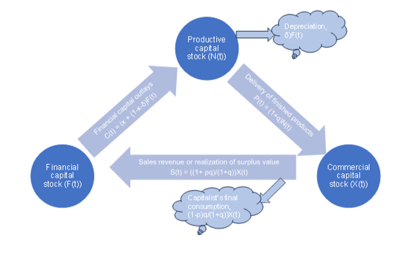
)In this setup, the financial capital outlays, C(t), becomes the sum of the two components of financial expenditures, one for purchasing constant capital stock, κF(t) and the other for buying labor power, net of depreciation cost, (1-(κ+δ))F(t). Similarly, the production and delivery of finished products to the commercial capital stock contains the increment in value qN(t). Finally, the flow of the sales revenue consists of the recovery of the previous capital stock, (1/(1+q)X(t), the new financial commitment of realized surplus value to the financial capital stock, (pq/(1+q))X(t), and the last portion that leaks from the circuit for the capitalist’s final consumption, ((1-p)q/(1+q))*X(t).
The rate of change in the productive capital stock at time t, dN/dt is a function of the corresponding inflow, C(t) and outflow, P(t). The rate of change in the commercial capital stock at time t, dX/dt is also a function of the difference between P(t) and S(t). Finally, the change in the financial capital stock at time t, dF/dt is an increasing function of S(t) net of the capitalist income for final consumption, ((1-p)q/(1+q))*X(t), and a decreasing function of the financial capital outlays, C(t). Therefore, the relevant system of differential equations becomes the following (see also Figure 3-1):
N
t
X
t
F
t
(
2
)Figure 3-1 A diagram for a modified circuit of capital model without time-lags
The identification of the injection and leakage variables and the derivation of the two class incomes
The identification of the injection and leakage variables and the derivation of the two class incomes
There are two leakage variables in this model. The first one is total cost of depreciation of the productive capital stock, δ*F[t] and the other the capitalist’s income for final consumption, (1-p)q/(1+q))*X(t). The injection variable is the capitalized realized surplus value, pq/(1+q)*X(t) that is reentering the circuit for the next round of the production. If the injection variable is greater than the sum of the two leakage variables, the circuit of capital will grow continuously. On the other hand, if the sum of the two leakage variables is greater than the capitalized surplus value, the system will shrink over time.
The financial capital outlays, C(t) consists of a portion that is used to purchase constant capital and the other portion tied to purchasing labor power. The exact proportion is determined by the technical composition parameter, κ, plus the depreciation rate of constant capital, δ. Therefore, if κF(t) represents the financial expenditure tied to fixed manufactured capital stock, the remaining (1-κ-δ) F(t) becomes total cost of buying labor power, which is simply the same as labor income for workers (LI(t)). Finally, given the portion of capitalized surplus value, pq/(1+q))X[t], we can also determine other portion that is leaked from the circuit for meeting the need of the capitalist’s final consumption, (1-p)q/(1+q))X[t]. This is the capitalist income for final consumption (CIFC(t)). In this way, we can derive the following two distinct social class incomes from the circuit of capital model:
LI[t]=(1-κ-δ)F(t)CIFC[t]=(1-p)q/(1+q))[t]
(
3
)Merits and limitations of the model and the specification of time-lags
Merits and limitations of the model and the specification of time-lags
Simulations of the simple reproduction of the model with and without time-lags
Simulations of the simple reproduction of the model with and without time-lags
A simple reproduction of the model without time-lags
A simple reproduction of the model without time-lags
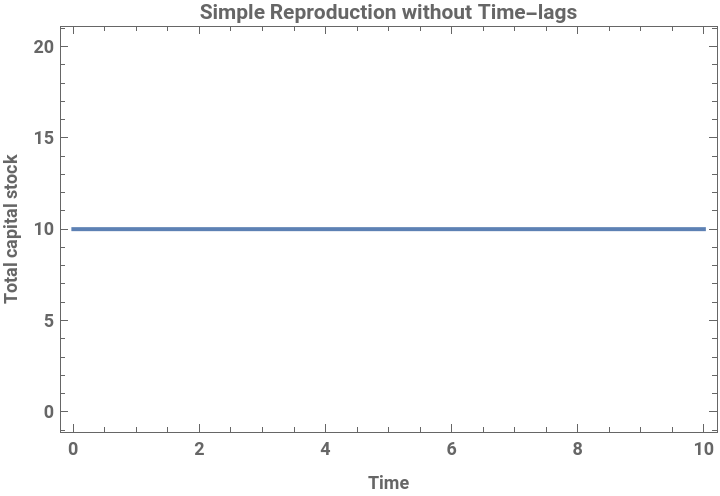
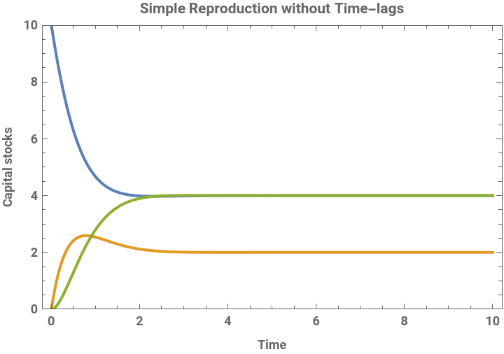
What will be the solution to this system of differential equations? For an illustration purpose, let us visualize the solution curves of the three capital stocks assuming that there is no increase in the financial capital stock. If we assume that the depreciation of the productive capital stock is negligible (δ = 0), this simple reproduction of the model without time-lags can be simulated by setting the capitalization rate equal to zero, p = 0. Assuming that the technical composition parameter, κ = 0.5, the surplus value, q = 100% (q =1), with initial value of the financial capital stock, F(0) = 10, while both the productive and commercial capital stock, N(0) = X(0) = 0, we can get the following result:
Clear[eqns,FCS,PCS,CCS,FCS0,PCS0,CCS0,sol,t,κ,δ,p,q];eqns={FCS'[t]==(1+p*q/(1+q))*CCS[t]-(κ+(1-κ-δ))*FCS[t],PCS'[t]==(κ+(1-κ-δ))*FCS[t]-(1+q)*PCS[t],CCS'[t]==(1+q)*PCS[t]-((1+(p*q)+(1-p)*q)/(1+q))*CCS[t],FCS[0]==FCS0,PCS[0]==PCS0,CCS[0]==CCS0};κ=0.5;δ=0.0;p=0.0;q=1;FCS0=10;PCS0=0;CCS0=0;sol=NDSolve[eqns,{FCS[t],PCS[t],CCS[t]},{t,0,100}];
In[]:=
Plot[Evaluate[FCS[t]+PCS[t]+CCS[t]/.sol],{t,0,10},Frame->True,FrameLabel->{"Time","Total capital stock"},PlotLabel->"Simple Reproduction without Time-lags",LabelStyle->Directive[Bold]]Plot[Evaluate[{FCS[t],PCS[t],CCS[t]}/.sol],{t,0,10},PlotRange->{0,10},PlotLegends->{"Financial capital stock","Productive capital stock","Commercial capital stock"},Frame->True,FrameLabel->{"Time","Capital stocks"},PlotLabel->"Simple Reproduction without Time-lags",LabelStyle->Directive[Bold]]Plot[Evaluate[{(1-κ-δ)*FCS[t],((1-p)*q/(1+q))*CCS[t]}/.sol],{t,0,10},PlotRange->{0,10},PlotLegends->{"Labor income","Capitalist income for final consumption"},Frame->True,FrameLabel->{"Time","Relative incomes"},PlotLabel->"Simple Reproduction without Time-lags",LabelStyle->Directive[Bold]]
Out[]=
Out[]=


Out[]=
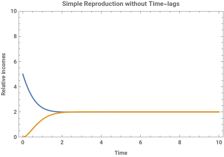
At the beginning, the financial capital stock decreases as it is expended to set up and organize the production activity. The productive capital stock, in turn, initially increases and reaches its peak as finished products are delivered to the node of the commercial capital stock. The realized surplus value contained in the sales revenue leaks out from the circuit in the form of the capitalist income for final consumption. Therefore, the total capital stock remains the same as before. The labor income falls from its initial value (kappa*F(0) = 0.5*10 = 5) and converges the capitalist income for final consumption ((1-p)q/(1+q)*X(t) = 1*1/2*5 = 2).
A simple reproduction of the model with time-lags: The case when Tf = Tp = Tc = 2
A simple reproduction of the model with time-lags: The case when Tf = Tp = Tc = 2
Using the same parameter and initial values above, we can also run the simulation for the simple reproduction of the model adjusted by the three time-lags. This time, however, suppose first that the three time-lags are evenly increased from zero to two. That is, Tf = Tp = Tr = 2. If the three time-lags are evenly increased in this way, the speed of the adjustment among the three capital stocks slows down proportionately. The speed of the distribution of the two social class incomes is also reduced in tandem. The higher the value of the time-lags, the lower and slower the volume and accumulation of the three capital stocks.
A simple reproduction of the model with time-lags: The case when Tf > Tp >Tc ≥ 0
A simple reproduction of the model with time-lags: The case when Tf > Tp >Tc ≥ 0
In contrast, if there are uneven changes among the three time-lags, for example, Tf = 2, Tp = 1, and Tr = 0, the pattern of the interaction among the three capital stocks is fundamentally altered, so is the level and distribution pattern of the two class incomes.
Comparative dynamic analyses of the expanded reproduction case with uniform changes in time-lags
Comparative dynamic analyses of the expanded reproduction case with uniform changes in time-lags
Comparative dynamic analyses of the expanded reproduction case with uneven changes in time-lags
Comparative dynamic analyses of the expanded reproduction case with uneven changes in time-lags
Introduction
Introduction
One important issue at hand is whether can continue to use the Marxian circuit of capital model to account for financialization phenomena and recurrent realization crises under capitalism. Financialization has been used to describe excessive growth of the financial sector vis-a-vis the rest of the economy. The proliferation of various financial instruments (‘fictitious capital’) that do not directly contribute to the production activity and the greater dependency of non-financial corporate business management on the vagary of financial portfolio investment are some of stylized facts of this phenomenon (Palley 2012, 2013; Stockhammer 2008; Stockhammer et al 2011). The term realization crisis refers to the case when produced commodities are not sold on the product market as intended, thereby substantially lowering the size of capitalized surplus value in the circuit. In the absence of offsetting mechanisms that absorb the portion of excess supply of commodities via extended credit or the Keynesian aggregate demand management, for example, the involuntary inventory slows down the accumulation of the productive capital stock in the economy. This section attempts to extend the circuit of capital model to explain these phenomena.
The effect of financialization
The effect of financialization
Scenario
Scenario
Financialization in this model setting can be perceived as a reduction in the total financial capital outlays that could be otherwise used for financing the operation of the productive capital stock. If we ignore the financial time-lag, this phenomenon can be captured by a reduction in the total financial capital outlays for production. Therefore, we can modify the differential equation of the productive capital stock as dN/dt = (κ-α + (1-κ-α-δ))F[t]/(1+Tf) - (1+q)N[t]/(1+Tp) where the parameter α represents this reduction.
In the time-lags adjusted model, however, the same phenomenon can be perceived as the lengthening time-lag tied to mobilizing financial capital outlays. Therefore, the effect of financialization on the accumulation of the three capital stocks as well as on the two derived income variables can be captured by the simulation result with a greater value of Tf. The substantial increase in the financial time-lag, Tf, while all other initial conditions and parameters remain the same as before, represents the effect of the substantial delay in mobilizing and expending the financial capital stock available to finance the operation of the productive capital stock and the dynamic interactions among the three capital stocks over time. In order to highlight the effect of this change, we can set Tp = 0, Tf = 2, and Tx = 0, while all other initial conditions and parameters remain the same as before. That is, N[0] = X[0] =0, F[0] = 10, and κ = 0.5, δ = 0.0, p = 0.5, and q = 1.
A visualization of the model solution
A visualization of the model solution
The simulation result shows that the total capital stock continues to grow. However, the composition of the source of the growth of the total capital stock is altered: the financial capital stock accumulates more relative to the other two capital stocks. Alternatively, we can say that it takes longer time for the financial capital stock to organize the production activity. This means that the greater proportion of the financial capital stock is retained rather than being immediately used to finance the operation of other capital stocks. Consequently, the speed of the accumulation and the volume of both the productive and commercial capital stock remain sluggish.
It is also important to note that the total labor income is reduced under this scenario. As a greater portion of the financial capital stock is diverted away from the production activity, the total financial capital outlays that could have been otherwise used to finance the labor cost is reduced. On the other hand, there is no visible sign that shows the growth rate of capitalists’ income for final consumption is negatively affected by this phenomenon, even though there may be some negative level effects in the long run.
The effect of realization crisis
The effect of realization crisis
Scenario
Scenario
The effect of the realization crisis can be captured by a decrease in realized surplus value. In the model without time-lags, this reduction is indicated by either (1) lowering the value of the realized surplus value parameter, q, or (2) subtracting a certain portion from dF/dt. In other words, we can modify the differential equation for the financial capital stock as dF/dt= (1+p*(q- β)/(1+q))*X[t]/(1+Tr) - (κ + (1-κ-δ))*F[t]/(1+Tf) where the newly introduced parameter β captures the effect of involuntary accumulation of inventory on the change in the financial capital stock. If we assume that the capitalization ratio remains the same as before, the decrease in the value of realized surplus value will lower the growth of total financial capital stock out of which a certain portion will be expended to finance the operation of the productive activity in the next round of the circuit.
In our current model with time lag, we can think of the same phenomenon as lengthening the time lag associated with the transformation of the commercial capital stock into the financial capital stock. The increase in the value of the commercial time-lag, Tr, represents the substantial delay in selling produced commodities, which is precisely the same effect of the accumulation of involuntary inventory. To highlight this effect in the simulation, we set Tp = Tf = 0, and Tr = 2, while letting all other parameters and initial conditions remain the same as before. That is, N[0] = X[0] = 0, F[0]=10, and κ = 0.5, δ = 0.0, p = 0.5, and q = 1.
A visualization of the model solution
A visualization of the model solution
The simulation result shows that the speed of the growth of the total capital stock slows down. More importantly, the composition of the source of growth is also altered: this time, the commercial capital stock is accumulated more relative to the other two capital stocks. Alternatively, we can say that it takes longer time to sell the finished product than before. Therefore, the level and speed of the accumulation of the three capital stocks is lowered substantially. In addition, the variable for the capitalists’ income for final consumption is negatively affected by the delay in sales.
An interactive visualization with varying parameters and time-lags
An interactive visualization with varying parameters and time-lags
Before closing, let us finally attempt to visualize the effect of the change in the parameters and time-lags on the accumulation of the three capital stocks interactively. The following syntax can show this dynamic behaviors:
Conclusion
Conclusion
The Marxian circuit of capital model is an important analytical framework that allows us to examine the process of capital accumulation, while keeping track of interactions among the productive, commercial, and financial capital stock via three corresponding flows. The model also allows us to identify two distinct sources of social-class income for both wage laborers and capitalists and to examine how their respective incomes change as the three capital stocks accumulate.
In this paper and notebook, we have shown how we can formally set up, solve, and visualize the circuit of capital model with varying parameter values. The solution curves from both simple reproduction and expanded reproduction case are visualized with and without uniform changes in time lags. We have also run multiple simulations to capture the effect of the change in some crucial parameters such as technical composition ratio of capital, surplus value, and capitalization ratio, with both uniform and uneven changes in time lags. The interactive graphics allows us to simulate and visualize the adjustment pattern as well.
Reference
Reference
Hee-Young Shin. 2023. “A computational approach to the Marxian circuit of capital model”, SSRN (https://papers.ssrn.com/abstract=4304658)
CITE THIS NOTEBOOK
CITE THIS NOTEBOOK
A computational approach to the Marxian circuit of capital model
by Hee-Young Shin
Wolfram Community, STAFF PICKS, August 25, 2023
https://community.wolfram.com/groups/-/m/t/2998966
by Hee-Young Shin
Wolfram Community, STAFF PICKS, August 25, 2023
https://community.wolfram.com/groups/-/m/t/2998966