Intro
Intro
The problems of choice, preference criteria, and decision-making have always been a complex and ambiguous topic.
Currently, the field is heavily used in neural networks and AI.
But there is a simple geometric structure (that fits perfectly with Mathematica),
allowing to look at the questions of choice and preference in an unusual and deep way.
This is the task of evenly distributing centers in some region.
We can imagine that the region is some field of life or science.
Or our resources.
How many centers does it take to optimally control (or study) this area?
How to place them? What are the selection criteria?
There are several simple and obvious approaches, but when analyzed in detail, they reveal many paradoxes and contradictions.
First, I would like to look at a structure known as the centroidal Voronoi tesselations.
dingbat and brown frame means initialization cells and
★ dingbat and gray frame means cells need to run.
★ dingbat and gray frame means cells need to run.
Definitions
Definitions
It is important to distinguish carefully concepts: region, points (of region), seeds, cells and centroids.
◼
Voronoi tesselation
The Voronoi mesh consists of convex cells, each associated with a seed and defined by , which is the region of points closer to than any other seed for .
n
p
i
pd(,p)≤d(,p)
∧
1≤j≤n∧j≠i
p
i
p
j
p
i
p
j
j≠i
◼
Centroidal Voronoi tesselation
A centroidal Voronoi tessellation is a VT whose seeds are the
centroids (centers of mass) of the corresponding Voronoi cells.
centroids (centers of mass) of the corresponding Voronoi cells.
◼
Stable and unstable CVT
On a simple level, if we apply any searching algorithms, they will converge to stable CVT (even with minor errors).
From unstable CVT the algorithm will always deviate.
From unstable CVT the algorithm will always deviate.
Lloyd relaxation algorithm for SCVT
Lloyd relaxation algorithm for SCVT
Although for a large number of centers this algorithm is not the most effective
it is quite suitable for our purposes. As a result of tests, I came to the conclusion,
that the optimal implementation of a Lloyd’s for Mathematica ≥ 14.2 is the following package:
it is quite suitable for our purposes. As a result of tests, I came to the conclusion,
that the optimal implementation of a Lloyd’s for Mathematica ≥ 14.2 is the following package:
Clear[arrDistC,lloydStepOrdered];(*Distancebetweenarraysofpoints*)arrDistC=Block{nf},Compile{{arr1,_Real,2},{arr2,_Real,2}}, (nf=Nearest@arr1;Total[EuclideanDistance[First@nf@#,#]&/@arr2]);(*MainLloydstepwithorderingcells*)lloydStepOrdered[pts_]:=Block[{m={VoronoiMesh[pts,{{0,1},{0,1}}],2}},AnnotationValue[m,MeshCellCentroid][[NearestMeshCells[m,#][[1,2]]&/@pts]]];(*Lloydprocess:stopafter!!!or!!!*)lloydProc[pts_,tol_,maxIt_]:=NestWhile[lloydStepOrdered@#&,pts,arrDistC@##>tol&,2,maxIt];(*Graphics*)voronPlot[pts_,size_:70]:=With{mesh=VoronoiMesh[pts,{{0,1},{0,1}}]},GraphicsEdgeForm@Black,FaceForm@DarkGray,mesh, StandardOrange,PointSize@.06,Point@pts,ImageSizesize;pattsCompare[pts1_,pts2_]:=Graphics[{EdgeForm@Black,FaceForm@DarkGray,Rectangle[],StandardRed,PointSize@.07,Point@pts1,Black,PointSize@.03,Point@pts2},ImageSize->130];
Test experiment
Test experiment
Let’s run the process 10-15 times for a small number of seeds e.g. 7,
starting with random array of points and look at the results.
starting with random array of points and look at the results.
★
In[]:=
numTries=10;numSeeds=7;data=ParallelTable[lloydProc[RandomReal[{0,1},{numSeeds,2}],,],{numTries}];Grid[Partition[voronPlot/@data,5]]
-5
10
3
10
Out[]=
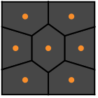
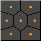
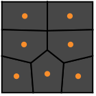
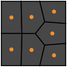
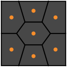
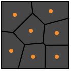
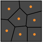
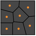
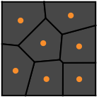
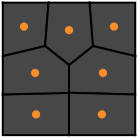
What do we see?
1. The CVT patterns are indeed (intuitively) evenly distributed over square region,
controlling each cell, as it were.
2. The algorithm converges to different patterns.
3. If we look closely, we will see that many of them match up with accuracy before rotations and reflections.
However, some of them fundamentally different.
For 7 seeds, there must be exactly three species. If you haven’t found them =) start the process again.
Detecting patterns
Detecting patterns
Of course, we are interested in configurations that are topologically different in structure.The task of recognizing patterns (including rotated, reflected, scaled; audio, video, etc.) has now been solved very effectively by the networks and AI.I decided to go straight, old-fashioned way, to understand the phenomenon deeply.Is known that the equal patterns of seeds in the square must be invariants of the so-called dihedral group- Wiki 2- Wolfram demonstrationsThis group has 3 generators: - Identity ℯ- Rotation by 90° counterclockwise - Reflection about the diagonal joining vertices “2” and “4” and 8 independent elements If two patterns mapped by any of these elements, they are equal as centroids of the square.
ℯ,,,,,,,
2
3
2
3
Unfortunately, the built-in FindGeometricTransform works very poorly with such a group.
Although I may not have managed to use it properly.
In any case, we will continue our detailed analysis and implement the dihedral group transformation:
Although I may not have managed to use it properly.
In any case, we will continue our detailed analysis and implement the dihedral group transformation:
In[]:=
Clear[dihedralTrans];dihedralTrans=Join RotationTransform[#,{.5,.5}]&/@{0,π/2,π,-π/2}, ReflectionTransform[#,{.5,.5}]&/@{{-1,1},{1,0},{1,1},{0,1}} ;
Because we don’t know how points "melt," to test the equivalence of patterns in the sense of group, we will have to apply all transformations for one pattern and compare it with another (for example, by calculating the sum of the distances between the nearest points)
In[]:=
Clear[patternDist];patternDist[arr1_,arr2_]:=With{trans=Through[dihedralTrans[arr2]]}, Min[arrDistC[arr1,#]&/@trans]/;MatrixQ[arr1,NumericQ]&&MatrixQ[arr2,NumericQ];
Let’s get enough SCVT examples to assume numSeeds = 7 and see,
what the distance between patterns statistics look like:
what the distance between patterns statistics look like:
★
In[]:=
Clear[data,distData];Block{numTries=150,numSeeds=7,tol=,maxIters=},data=ParallelTable[lloydProc[RandomReal[{0,1},{numSeeds,2}],tol,maxIters],{numTries}];distData=ParallelTable[patternDist@@First@Subsets[data,{2},{s}],{s,Binomial[numTries,2]}];Histogram[distData,{Min@distData,Max@distData,.01},PlotInteractivity->False,PlotLabel->Row@{"Distances between CVT patterns for ",numSeeds," seeds"}]
-5
10
5
10
Out[]=
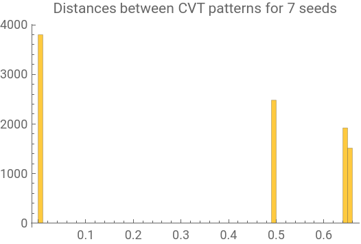
In this case, the picture is clear. There are cluster of very small distances which (with accuracy to calculation error) indicate that the patterns match. We can find the upper bound of this cluster (for numSeeds = 7, it’s about ) and distinguish truly different patterns
(labeled with population):
-4
10
(labeled with population):
★
In[]:=
Block[{δ=Sort[Flatten[MinMax/@FindClusters[distData,2,Method->"KMeans",PerformanceGoal->"Speed"]]][[2]]},Row[voronPlot@#[[1]]&/@Tally[data,patternDist[#1,#2]<δ&]]]
Out[]=
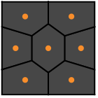
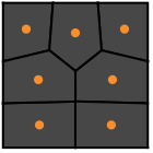
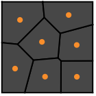
On one hand, it is obvious that they are topologically distinct and include all possible SCVTs for numSeeds = 7 (?).
I even posted the OEIS sequence hoping to conduct a classification of CVT at least up to a number of seeds less than 50.
I even posted the OEIS sequence hoping to conduct a classification of CVT at least up to a number of seeds less than 50.
However, things have been much more complicated than they seem.
1. Are 100 random initial configurations enough to find all possible patterns?
How much effort does it take to be sure?
2. Which configuration is "better" in the sense of distribution evenness?
Lloyd’s algorithm itself does not provide such a criterion.
3. Finally, with the increase number of seeds there is a more complex problem of choice,
which we will discuss further.
Decision problem
Decision problem
If we repeat the experiment for more centers, such as numSeeds = 17,
histogram of distances will become more vague:
histogram of distances will become more vague:
Note the cluster near distance 0.22.
What are the configurations that make up these distances relative to the dihedral group?
Select a pair, restore the appropriate transformation and compare the two visually:
side by side and overlapping
What are the configurations that make up these distances relative to the dihedral group?
Select a pair, restore the appropriate transformation and compare the two visually:
side by side and overlapping
Some preview
Some preview
However, in the course of my research I have explored a fundamentally different approach to analyzing the distribution of centers: energy optimization. It provides an answer to the question of the qualitative difference of the patterns.
Best of all, it can detect and analyze unstable CVT.
It will be discussed in the next post.
Best of all, it can detect and analyze unstable CVT.
It will be discussed in the next post.
CITE THIS NOTEBOOK
CITE THIS NOTEBOOK
Centroidal Voronoi tessellations counting and decision making
by Denis Ivanov
Wolfram Community, STAFF PICKS, May 19, 2026
https://community.wolfram.com/groups/-/m/t/3718065
by Denis Ivanov
Wolfram Community, STAFF PICKS, May 19, 2026
https://community.wolfram.com/groups/-/m/t/3718065