A cellular automaton (CA) is a grid of simple cells that all update in parallel according to one fixed rule. This notebook asks whether a rule can make a 2D CA grow into a circle after a fixed number of steps. Because the rule space is enormous, adaptative evolution based search is an interesting alternative, in this work we explore four adaptive search strategies like hill climbing, (μ,λ) population evolution strategy, island model with migration, and a sexual genetic algorithm are compared on the same fitness evaluation budget. The goal is not only to find circular rules, but to study the power of the evolution process in order to achieve an objective. Interestingly, we found that there is not a significant difference between the different evolution strategies. This suggest that particular implementation of adaptative evolution is not as important as the way you define your particular fitness function.
Introduction
Introduction
What Are Cellular Automata?
What Are Cellular Automata?
A cellular automaton is one of the simplest possible programs: a grid of cells, each in one of a finite number of states, that updates in discrete steps according to a local rule. Yet as Stephen Wolfram explored in A New Kind of Science, even these minimal systems can produce behavior of remarkable complexity. The key insight is that complexity does not require complicated underlying rules; it can emerge from the iterated application of something very simple.
In our two-dimensional setup, each cell looks at its neighbors in a rectangular neighborhood and decides its next state based on the total of those neighbor values. This is the so-called totalistic rule family. We initialize the grid with a single active cell at the center and let the automaton evolve for a fixed number of steps. The question we ask is: can we find a rule that makes the resulting pattern look like a circle?
Because the space of possible rules grows exponentially with the number of colors and the range of the neighborhood, we cannot simply enumerate all possibilities. This is where computational irreducibility enters the picture: there is no shortcut to knowing what a given rule will do without explicitly running it.
Looking at the behavior of an example 2D cellular automata we can readily see the complex behavior. In the animation bellow you can see the progression across time.
Evolve a simple 2D totalistic CA from a single active cell:
Out[]=
Why the Rule Space Is Too Large to Search Exhaustively
Why the Rule Space Is Too Large to Search Exhaustively
We use two-dimensional totalistic CAs. At each step a cell's new color depends only on the total of its neighbors' colors and its own. With a 3x3 Moore neighborhood there are 9 cells, so the possible sums range from 0 to 9(k-1). That gives 9(k-1)+1 rule cases, and each case can output any of k colors.
Totalistic Rules and the Size of Rule Space
Totalistic Rules and the Size of Rule Space
A totalistic rule means that the next state of a cell depends only on the sum of its neighbors' states, not on their exact spatial arrangement. This is a significant simplification compared to outer-totalistic or general rules, but it still leaves us with a vast search space. For our chosen configuration with k=4 colors and range r={1,1}, the neighborhood contains 9 cells.
9(k-1)+1
k
Display the number of rule cases and possible rules for a few values of k:
k | rule cases | possible rules |
2 | 10 | 1024 |
3 | 19 | 1162261467 |
4 | 28 | 72057594037927936 |
For k=4 the space already contains about rules. That is why we turn to evolutionary search instead of enumeration.
7.2
16
10
Compute the exact size of the k=4 rule space:
In[]:=
=[4^(9*(4-1)+1)]
Out[]=
72057594037927936
Defining Circularity : A Fitness Function
Defining Circularity : A Fitness Function
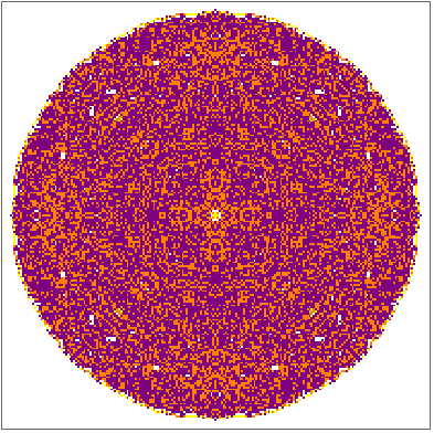
How do we tell a computer that one pattern is more circular than another? Our approach is geometric. The fitness function measures how close the final pattern is to a perfect circle. The CA is run for 100 steps from a single central cell, the outer contour is extracted, and the distances from each contour point to the center are collected. A perfect circle would have zero spread in those distances.
Show the final state of a good rule and its fitness value:
Out[]=
,fitness = 58.2
Here is the detailed description of how fitness is calculated
Extract the outer contour from the final state:
In[]:=
contour = N@Catenate[MapIndexed[Function[{val, idx}, {idx[[1]], #} & /@ val], nonzeroRange /@ state]];
Length[contour]
Length[contour]
Out[]=
402
Each contour point is a {row, column} pair. From the center of the matrix we compute the Euclidean distance to every contour point. The mean of those distances is the average radius, and the standard deviation tells us how irregular the shape is.
Compute mean radius and standard deviation manually:
In[]:=
centro = Dimensions[state]/2.;
distancias = Sqrt[Total[(contour - ConstantArray[centro, Length[contour]])^2, {2}]];
{Mean[distancias], StandardDeviation[distancias]}
distancias = Sqrt[Total[(contour - ConstantArray[centro, Length[contour]])^2, {2}]];
{Mean[distancias], StandardDeviation[distancias]}
Out[]=
{99.2525,0.705423}
The fitness score is defined as MeanRadius / (StdDev + 1). Adding 1 prevents division by zero and keeps the score meaningful when the standard deviation is very small. A larger value means a more circular shape. The same quantities are returned by CircleMetrics.
The actual output of the CircleMetrics function builtin in the package:
In[]:=
CircleMetrics[state]
Out[]=
MeanRadius99.2525,StdDev0.705423,Fitness58.1982,Circularity99.2943,DeviationPct0.710735,Area41019
Here fitness is defined as the mean radius divided by the standard deviation plus one. Larger values mean a better circle.
For clarifying purposes an animation based on how the fitness is calculated you can find in the package the next function, that produces an animation based on the fitness calculation process.
Generate an animation that shows how the ideal-circle overlay, contour, and radius statistics are built step by step:
In[]:=
FitnessAnimationForRule[{489833929985643,{4,1},{1,1}},100]
Out[]=
fitness_animation_rule_489833929985643.gif
In[]:=
Out[]=
The gap between distances is due to the fact the algorithm detects the boundary in a row-wise fashion.
Mutation: One Digit at a Time
Mutation: One Digit at a Time
In the wolfram encoding, a totalistic rule is simply an integer. The genotype is the rule number; the phenotype is the two-dimensional pattern it produces after a fixed number of steps. Mutation operates at the genotype level.
All four search strategies move through the rule space via mutations. A rule is stored as an integer whose base-k digits are the outputs of the rule table. Our mutation function picks one digit at random and changes it to a different value. For k=4 a single mutation changes one entry of the rule table.
All four search strategies move through the rule space via mutations. A rule is stored as an integer whose base-k digits are the outputs of the rule table. Our mutation function picks one digit at random and changes it to a different value. For k=4 a single mutation changes one entry of the rule table.
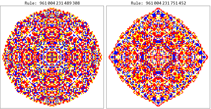
Compare the digits of a rule before and after one mutation:
Out[]=
original | 961004231489308 | {0,0,0,3,1,2,2,2,0,0,1,3,0,3,2,3,3,1,2,0,1,3,1,3,0,1,3,0} |
mutant | 961004231751452 | {0,0,0,3,1,2,2,2,0,0,1,3,0,3,2,3,3,1,3,0,1,3,1,3,0,1,3,0} |
Some of these genotypic changes also result in phenotypic changes, but this is not always the case.
Plot the two different rules one being the result of change in one digit the genotype of the other:
Out[]=
Search Strategies
Search Strategies
Now that we can measure how circular a cellular automaton is and introduce variations through mutation, we can start navigating the search space .The following sections outline different strategies for applying adaptive evolution.
Hill Climbing: A Greedy Adaptive Walk
Hill Climbing: A Greedy Adaptive Walk
What hill climbing does
What hill climbing does
Hill climbing is the simplest adaptive search. It starts from a random rule and repeatedly applies a one-digit mutation. If the mutant has higher fitness, the search moves to it; otherwise it stays where it is. Because it only accepts improvements, it quickly reaches a local optimum. That is why the search is run many times from different random seeds; each replicate is an independent walk, and the best result across all replicates is kept.
Fitness is evaluated only at the 100th step, not at every intermediate step, because the goal is a target shape and this keeps the search affordable.
Run a hill-climbing search (Code cell provided for re-use):
In[]:=
resHCcomp = SearchHillClimbing["k" -> kComp, "r" -> rComp, "FinalStep" -> pfComp,
"ReplicateSize" -> 20, "Generations" -> 1000, "MaxEvaluations" -> 20000,
"MaxDeviation" -> dmaxComp, "StoreEvolutionStates" -> True,
"Verbose" -> True, "SearchMode" -> "Random", "TimeLimitMinutes" -> 20,
"Parallel" -> True, "ProgressFrequency" -> 1, "AutoVisualize" -> False];
"ReplicateSize" -> 20, "Generations" -> 1000, "MaxEvaluations" -> 20000,
"MaxDeviation" -> dmaxComp, "StoreEvolutionStates" -> True,
"Verbose" -> True, "SearchMode" -> "Random", "TimeLimitMinutes" -> 20,
"Parallel" -> True, "ProgressFrequency" -> 1, "AutoVisualize" -> False];
A single greedy walk easily gets stuck, so the search is run in blocks called replicates. Each replicate receives a different random seed, which means a different random starting rule and a different path through the rule space.
The code below loads a pre-computed run for the visualizations in this section.
Load the pre-computed hill-climbing run:
In[]:=
normHCcomp = ImportString[FromCharacterCode[Normal[BaseDecode[hcRunMX]], "ISO8859-1"], "MX"];
Here is the best rule found and its 100th state, overlaid with the ideal circle.
Visualize the best rule with the ideal-circle overlay:
The 2D temporal progression shows how the pattern is assembled step-by-step.
Show the 2D temporal evolution of the best rule:
The mutation-detail plot shows the actual digit changes along the best replicate and each CA at step 100. Each strip is the full 28-digit rule at one improving step; the colored cell marks the digit that changed.
Display the digit changes along the best replicate:
The broader mutation view places each improved organism next to its final-state phenotype at step 100, with the number of generations between breakthroughs and drawing the ideal circle over the CA.
Show the organisms that formed breakthroughs and the generations between them:
The path plot tracks circularity across all replicates. Red points are rejected organisms, the red line shows the best fitness overtime, and the small CA thumbnails mark breakthrough rules.
Plot circularity paths with breakthroughs and failed attempts:
It’s interesting to note in this evolutionary path how there are also micro-improvements in the previous graph.
The evolutionary process can be better seen if we graph the tree of cellular automata and the rejected attempts as well as the accepted evolutionary path; below it can be seen at a glance how the initial CA starts with a clearly rectangular shape and gradually acquires a smooth and rounded shape.
Draw the graph of improving rules for one replicate:
(μ, λ): A Population of Mutants
(μ, λ): A Population of Mutants
The (mu, lambda) evolution strategy
The (mu, lambda) evolution strategy
An evolution strategy maintains a small population of μ parent rules. In each generation it creates λ offspring by mutating randomly chosen parents. Only the best μ offspring survive and become the parents of the next generation. This is selection by truncation: the population constantly moves toward higher fitness, but because several offspring are tested each generation it can explore a wider neighborhood than a single greedy walk.
The ratio λ/μ is often around 5; here μ=20 and λ=100.
Run a (μ, λ) search (Code cell provided for re-use):
In[]:=
resMLcomp = SearchMuLambda["k" -> kComp, "r" -> rComp, "FinalStep" -> pfComp,
"Mu" -> 20, "Lambda" -> 100, "Generations" -> 200,
"TimeLimitMinutes" -> 20, "MaxDeviation" -> dmaxComp,
"StoreEvolutionStates" -> True, "Seed" -> 189952,
"Verbose" -> True, "AutoVisualize" -> False];
"Mu" -> 20, "Lambda" -> 100, "Generations" -> 200,
"TimeLimitMinutes" -> 20, "MaxDeviation" -> dmaxComp,
"StoreEvolutionStates" -> True, "Seed" -> 189952,
"Verbose" -> True, "AutoVisualize" -> False];
Selection is by ranking: after all offspring are evaluated, everyone is sorted by fitness and the top μ are kept. The code below loads a pre-computed run.
Load the pre-computed (μ, λ) run:
The best rule at the 100th step is presented below.
Visualize the best rule found by the population-based search:
Show the 2D temporal progression of that rule:
In[]:=
Visualize[normMLcomp, "Evol2D", "ShowIdealCircle" -> True]
The scatter plot below shows the population at each generation. Each point is one individual, positioned by its circularity and deviation. Over time the cloud drifts toward the upper-left corner: high circularity and low deviation. The best individual of each generation traces the red trajectory.
Plot the population path in circularity space:
The algorithm begins by generating an initial population of size μ. These represent the first “parents” in our search space. In the context of this cellular automaton framework, they are completely random totalistic rules. Each of these μ rules is evolved to the target timestep and evaluated to establish a baseline circularity fitness score.
Show the first narrative panel for one generation:
A second panel shows the same stage from a different angle, emphasizing how the next generation is selected.
Once the initial population is established, the evolutionary cycle drives forward by randomly sampling the μ parents and applying 1-bit mutation to each parent to generate a much larger pool of λ offspring, each of which is immediately simulated and evaluated for its circularity fitness. At the selection phase the entire previous generation of parents is discarded. The algorithm then ranks the λ newly evaluated offspring from best to worst and strictly selects only the top μ individuals to become the next generation of parents, forcing the population to continuously step forward into new areas of the search space.
Visualize the cartoon of the (μ, λ) population evolution strategy:
Show the grid of best individual generation-by-generation:
Plots circularity against generation :
We can also plot the genealogy of a sample of the population.
Plot the genealogy of the actual search showing the ancestors of each individual, and with a specific color the generation that he is from :
Island Model: Parallel Populations with Migration
Island Model: Parallel Populations with Migration
The island model splits the population into several isolated sub-populations. Each island evolves on its own for a number of generations, which lets different islands explore different regions of the rule space. Periodically, the best individuals migrate from one island to another, spreading good discoveries without collapsing diversity too quickly. This algorithm is analogous to how populations can separate and merge over time.
Here five islands of size 20 evolve for 20 epochs of 10 generations each.
Run an island-model search (Code cell provided for re-use):
In[]:=
resIslandsComp = SearchIslands["k" -> kComp, "r" -> rComp, "FinalStep" -> pfComp,
"NumIslands" -> 5, "PopSize" -> 20, "Epochs" -> 20,
"GenerationsPerEpoch" -> 10, "MaxDeviation" -> dmaxComp,
"TimeLimitMinutes" -> 20, "StoreEvolutionStates" -> True,
"Verbose" -> True, "AutoVisualize" -> False];
"NumIslands" -> 5, "PopSize" -> 20, "Epochs" -> 20,
"GenerationsPerEpoch" -> 10, "MaxDeviation" -> dmaxComp,
"TimeLimitMinutes" -> 20, "StoreEvolutionStates" -> True,
"Verbose" -> True, "AutoVisualize" -> False];
Within each island selection is by ranking: offspring are produced by mutating a random parent, then a certain number of individuals among parents and offspring are kept. Migration broadcasts the top migrants to every island, where they enter the next round of ranking.
Load the pre-computed island-model run:
The best rule and its temporal evolution.
Visualize the best island-model rule at the 100th progression step:
Show the 2D temporal progression of that rule:
A plot that visualizes how the initial population is established in each island:
Now we can show the changes to each island (y-axis) over time (x-axis):
Plot the per-island paths and circularity values with migration events marked with a gray dotted line:
In[]:=
Visualize[normIslandsComp, "IslandsPaths", "Metric" -> "Circularity",
"ShowPopulation" -> True, "MigrationLines" -> True]
"ShowPopulation" -> True, "MigrationLines" -> True]
Show the best organism of each island at sampled epochs:
Sexual Genetic Algorithm: Crossover and Tournament Selection
Sexual Genetic Algorithm: Crossover and Tournament Selection
Sexual reproduction combines genetic material from two parents. In this GA two parents are chosen by tournament selection (the best of three random candidates). With probability 0.7 a one-point crossover combines their base-4 digit strings; with probability 0.2 the child is further mutated. The operation is recorded as Crossover, Mutation, Crossover+Mutation, or Clone.
Run a sexual-GA search (Code cell provided for re-use):
In[]:=
resSexComp = SearchSexual["k" -> kComp, "r" -> rComp, "FinalStep" -> pfComp,
"PopSize" -> 200, "Generations" -> 200, "MaxDeviation" -> dmaxComp,
"StoreEvolutionStates" -> True, "TimeLimitMinutes" -> 30,
"Verbose" -> True, "AutoVisualize" -> False];
"PopSize" -> 200, "Generations" -> 200, "MaxDeviation" -> dmaxComp,
"StoreEvolutionStates" -> True, "TimeLimitMinutes" -> 30,
"Verbose" -> True, "AutoVisualize" -> False];
Crossover acts on the rule-table digits, not on individual bits. A random cut point splits the 28 digit positions; the child receives the first block from one parent and the remainder from the other.
Load the pre-computed sexual-GA run:
If crossover does not occur, the offspring is simply a direct clone of the first parent.
There is also possible that mutation happens. With a defined mutation probability, a single, randomly selected digit within the offspring’s genetic sequence is forcibly flipped to a new valid base-κ state. This means an individual can be the product of “Crossover + Mutation” inheriting a hybrid structure from two successful parents while simultaneously introducing a completely novel local dynamic that neither parent possessed.
There is also possible that mutation happens. With a defined mutation probability, a single, randomly selected digit within the offspring’s genetic sequence is forcibly flipped to a new valid base-κ state. This means an individual can be the product of “Crossover + Mutation” inheriting a hybrid structure from two successful parents while simultaneously introducing a completely novel local dynamic that neither parent possessed.
Show examples of crossover events during the first few generations:
Show an examples of Crossover+Mutation :
The best rule and its temporal evolution.
Visualize the best rule found by the sexual GA at the 100th progression step:
Show the 2D temporal progression of that rule:
The population scatter shows every evaluated organism projected by circularity and deviation. Failed attempts cluster near low circularity; the successful lineage climbs toward the upper-left corner.
Scatter the population by circularity and deviation:
In the previous plot it seems like the initial population has certain individuals very close to a perfect circle, however you can see that the average fitness value and its equivalent circularity measure is increasing.
The genealogy tree visualizes the complex ancestral lineage of the final best individual. Because the full evolutionary tree is excessively large, only the direct lineage leading to the best rule is shown. The diagram progresses downwards, depicting how multiple parent nodes from early generations converge into a single optimal solution at the bottom. Additionally, the nodes display visual phenotypes and are tagged with specific labels (such as C, CI, and C+M) to indicate the specific genetic operators applied during each generation, the green arrow means a crossover operation, purple means a crossover plus mutation operation, red means a only mutation process, gray means a clone from one of the parent.
Draw the lineage of the final best individual, every CA has the operation that produces himself R, Initialized randomly, C from crossover, Cl is clone, M for a single mutation, and C+M, mutation after crossover:
Making the nodes smaller we can see the best lineage with another layout:
Comparing the Four Heuristics
Comparing the Four Heuristics
◼
The common currency of the comparison: the number of fitness evaluations (the expensive operation) and the radial deviation in percent reached with them.
◼
For a controlled test, a benchmark was run separately: 5 paired runs per algorithm with an exact budget of 300 evaluations, every algorithm seeing the same random seeds, and the parameters of each algorithm scaled so that its maximum number of evaluations equals the budget.
The benchmark comparison (5 paired runs per algorithm, 300 evaluations each), embedded with Iconize:
Mean performance of each algorithm in the benchmark:
Best deviation so far against evaluation budget (median and quartile band over 5 runs, logarithmic scale):
Distribution of the final deviation for each algorithm:
Time and evaluations needed to reach each deviation threshold (k/n = how many of the 5 runs reached it):
Median time to reach each threshold (a missing bar means the algorithm never reached it):
◼
Reading of the results: all four strategies reliably reach a mean deviation of about 1% within 300 evaluations (islands 1.01%, (μ,λ) 1.11%, sexual 1.26%, hill climbing 1.40%). The ranking matters less than the similarity -- exactly Wolfram's conclusion that 'the details of how adaptive evolution is done don't matter much' (Wolfram, 2024a).
◼
Note on time vs. evaluations: hill climbing is the slowest per evaluation in this benchmark (35 s mean vs. about 29--31 s for the others), so wall-clock time and evaluation count tell slightly different stories.
Other findings and gallery of circular cellular automates
Other findings and gallery of circular cellular automates
The rules below are a selection of those discovered across multiple independent runs of the four search methods described above. They are not the only good rules found, but they illustrate the range of circular shapes that emerge and a few curious behaviors that appear when the same fitness pressure is applied through different evolutionary strategies.
◼
Different runs find different rules that solve the same problem -- visibly different 'ideas' for making a circle, echoing Wolfram's observation that evolution 'invents many different mechanisms' for one objective (Wolfram, 2024b).
Next we have one of the rules found, adjusted to find a circle at step 100, is allowed to evolve until step 600 where you can see how its shape ceases to be circular. In fact, if we try to draw a circle for the distances of the contour, the possible circle includes sections outside the grid, so what we are seeing is the shape trying to be circular but on a grid that no longer allows a circle of that size.
Next we have one of the rules found, adjusted to find a circle at step 100, is allowed to evolve until step 600 where you can see how its shape ceases to be circular. In fact, if we try to draw a circle for the distances of the contour, the possible circle includes sections outside the grid, so what we are seeing is the shape trying to be circular but on a grid that no longer allows a circle of that size.
One discovered rule grown for 600 steps -- a textured but sharply circular disk:
Mean radius versus step for the rule 393184302949960 against cellular automata timestep:
The following are 9 rules found by performing searches with the different algorithms used in this work. It is interesting to analyze not only the resulting circular shape but also the intermediate steps and the strategies that these automata execute to maintain their smoothness and circularity.
Nine rules collected in using the search function provides in this essay, each grown from a single seed cell for 100 steps:
In[]:=
ofRules = {50603830369011260, 961004231489308, 393184302949960, 839011674994312, 511777427641928, 566705530581384, 416297579357960, 393192821745288, 533928170903112};
ofColors = {0 -> White, 1 -> Yellow, 2 -> Blue, 3 -> Red};
ofData = CellularAutomaton[{#, {4, 1}, {1, 1}}, {{{1}}, 0}, 100] & /@ ofRules;
ofColors = {0 -> White, 1 -> Yellow, 2 -> Blue, 3 -> Red};
ofData = CellularAutomaton[{#, {4, 1}, {1, 1}}, {{{1}}, 0}, 100] & /@ ofRules;
The final pattern (step 100) of each rule, labeled by rule number (colors as above):
The same exploration produced space-time voxel stacks -- 2D growth with one voxel layer per time step (yellow/blue/red = states 1/2/3) -- embedded with Iconize:
In[]:=
ofVoxels = ImportString[FromCharacterCode[Normal[BaseDecode[ofVoxelsMX]], "ISO8859-1"], "MX"];
The nine voxel stacks, each grown from a single seed cell:
A Cautionary Example: One Time Step Is Not Enough
A Cautionary Example: One Time Step Is Not Enough
Fitness measured only at the final step can be fooled. The rule below has 0.70% deviation at step 100, which looks excellent, but its MeanRadius oscillates wildly between a compact disk and a full-field flash. This is a limitation of the current fitness function and motivates multi-step or area-perimeter measures in future work.
Next, if the average radius of the distances is plotted against the timestep of the automata, it can be observed how it presents an oscillating behavior that, precisely because the evaluation of the fitness function is only performed at step 100, coincides with a very circular shape at that specific step, but maintains its oscillating behavior between a square and a circle.
Plot the MeanRadius trajectory of the unstable rule:
Concluding Remarks
Concluding Remarks
Acknowledgements
Acknowledgements
I would like to thank the staff of the Wolfram Summer School for their continuous support throughout this project. I am especially grateful to my mentor, Willem Nielsen, for his excellent guidance during this research program; his help in clarifying key concepts was essential to the success of this work. Finally, my sincere thanks to Stephen Wolfram for suggesting this fascinating research topic, as well as for the theoretical framework of computational irreducibility and the ruliad that inspired this investigation.
References
References
1
.S. Wolfram (2002), A New Kind of Science. Wolfram Media.
2
.3
.S. Wolfram (2024), Why Does Biological Evolution Work? A Minimal Model for Biological Evolution and Other Adaptive Processes, Stephen Wolfram Writings. URL.
4
.S. Wolfram (2024), Foundations of Biological Evolution: More Results & More Surprises, Stephen Wolfram Writings. URL.
5
.S. Wolfram (2025), What's Special about Life? Bulk Orchestration and the Rulial Ensemble in Biology and Beyond, Wolfram Institute. URL.
AI Disclosure
AI Disclosure
The following generative AI tools were used in this project: Kimi by Moonshot AI (model Kimi 2.7 Thinking). They were used for formatting code and building visualization functions. All code and written content was reviewed, understood and approved by the author.
CITE THIS NOTEBOOK
CITE THIS NOTEBOOK
Evolving Circles: Adaptive Search in a Cellular Automaton Rule Space
by Jhoan Eduardo Saldarriaga Serna
Wolfram Community, STAFF PICKS, July 16, 2026
https://community.wolfram.com/groups/-/m/t/3763335
by Jhoan Eduardo Saldarriaga Serna
Wolfram Community, STAFF PICKS, July 16, 2026
https://community.wolfram.com/groups/-/m/t/3763335