ABSTRACT (original article): Quantitative forecasting of average rainfall into the next season remains highly challenging, but in some favourable isolated cases may be possible with a series of relatively simple steps. We chose to explore predictions of austral springtime rainfall in SE Australia regions based on the surrounding ocean surface temperatures during the winter. In the first stage, we search for correlations between the target rainfall and both the standard ocean climate indicators as well as the time series of surface temperature data expanded in terms of Empirical Orthogonal Functions (EOFs). In the case of the Indian Ocean, during the winter the dominant EOF shows stronger correlation with the future rainfall than the commonly used Indian Ocean Dipole. Information sources with the strongest correlation to the historical rainfall data are then used as inputs into deep learning artificial neural networks. The resulting hindcasts appear accurate for September and October and less reliable for November. We also attempt to forecast the rainfall in several regions for the coming austral spring. CITATION (original article): Stjepan Marcelja (2024), Forecasting seasonal rainfall in SE Australia using Empirical Orthogonal Functions and Neural Networks, arXiv:2408.10550. https://doi.org/10.48550/arXiv.2408.10550
We describe a very accessible way to explore the possibilities of forecasting rainfall based on the ocean surface temperature data. Due to the favourable conditions during the austral winter, test forecasts of the spring rainfall with Mathematica neural network tools achieve surprising accuracy. More detailed journal preprint is available as arXiv:2408.10550
Background
Background
Improved seasonal forecasting of rainfall in agriculturally important regions of Southeast Australia, allowing for better crop planning and optimisation, would be of great benefit on both local and global levels. Such forecasting is predominantly based on the states of the surrounding oceans that slowly change on the seasonal scales and thus provide a basis for the predictions one season ahead of the present.
The skill of forecasting seasonal changes in the state of the oceans is rapidly increasing. Globally most important are the El Niño/Southern Oscillation (ENSO) events, where recent improvements in deep learning methods and dynamical modelling led to the greatly increased forecast horizon [1,2]. These advances open a wide scope for translating better understanding of ocean climate fluctuations into practical rainfall forecasting.
Here we use deep learning neural networks to extract information from different ocean climate indicators and obtain useful rainfall forecasts. The project consists of two parts. First, we need to find the times of the year and the ocean indicators that contain information about the future rainfall. The data is then used as an input into artificial neural networks that provide quantitative estimates of the rainfall, as measured by rain gauges.
Major climate indicators, ENSO and the Indian Ocean Dipole (IOD) are most predictable during the austral winter, when larger events form and become apparent. The predictability of rainfall in SE Australia depends on these drivers and follows the same seasonal pattern. With the present method best predictions are obtained in July and August for the agriculturally important spring months of September to November.
To describe the state of the oceans and obtain accurate forecasts, information contained in the ENSO and IOD indices is insufficient and needs to be supplemented by other data providing a more complete picture of the physical state of the oceans. We use sea surface temperatures (SST) at different positions in the oceans, gradients of SST and an expansion of SST maps into empirical orthogonal functions (EOF). The expansion reduces the full information contained in the SST spatial and temporal distribution into the time series of the strength of the orthogonal independent components. For this task, we used the very helpful software developed by Andrew Dawson (https://ajdawson.github.io/eofs/latest/).
Slow climate changes affect the dynamical relationships between the ocean climate and rainfall. With the present method, the useful length of annual time series in forecasting is restricted to a relatively short recent period and the inclusion of older data is not helpful. Most of the time we limited the input to the period 2000-2024.
Finding variables that contain information about future rainfall
Finding variables that contain information about future rainfall
The simplest indicator of predictability is the correlation coefficient. Presently we look for areas of the oceans where SSTs strongly correlate with the future rainfall. For example, if we wish to forecast springtime rain, we search for correlation with winter SSTs, checking month to month relationships.
The code for the example Image below extracts data from the very large Hadley centre SST file: Each ocean position is associated with a time series of year 2000 to 2024 July SSTs. Large file analysis and handling was performed using the Ferret software provided by the NOAA
(https://ferret.pmel.noaa.gov/Ferret/downloads/pyferret).
At each position the correlation between SSTs and the October rainfall is calculated and the results are shown in the plot.
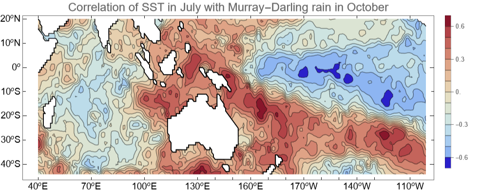
In Indian Ocean, the image shows a pattern of negative IOD (known to favour rain) and in the central Pacific a La Niña pattern (also known to favour rain). The strong feature east of the Australian continent is not mentioned in routine reports on climate indicators and we add it to the list of information sources for neural networks calculations.
A nonlinear indicator that measures the amount of information shared between the two variables is mutual information. In the next example we calculate mutual information between the central Pacific Niño3.4 area SSTs and the rainfall in Victoria for all month pairs in the period 2000-2024. The result will indicate which pairs share significant information. The code uses very useful EstimatedDistribution function:
In[]:=
Feature1=Nino24;Feature2=VictoriaRain24;(*indices:m1=>month1m2->month2g->year(1:24)*)MI2=Table[{0,0},{m2,1,12},{m1,1,12}];Do[PDF1[y_]=PDF[EstimatedDistribution[Feature1[[m1]],NormalDistribution[μ,σ]],y];PDF2[x_]=PDF[EstimatedDistribution[Feature2[[m2]],NormalDistribution[μ,σ]],x];data=Table[{Feature2[[m2]][[g]],Feature1[[m1]][[g]]},{g,1,24}];(*month1<->month12relationshipover24years*)Joint[x_,y_]=PDF[EstimatedDistribution[data,BinormalDistribution[{Subscript[μ,1],Subscript[μ,2]},{Subscript[σ,1],Subscript[σ,2]},ρ]],{x,y}];MI2[[m1,m2]]=NIntegrate[Joint[x,y]Log[Joint[x,y]/(PDF1[y]PDF2[x])],{x,-100,100},{y,-2,2}],{m2,1,12},{m1,1,12}];
Label1="Niño3.4 (month)";Label2="Victoria rain (month)";ListContourPlotMI2,InterpolationOrder1,
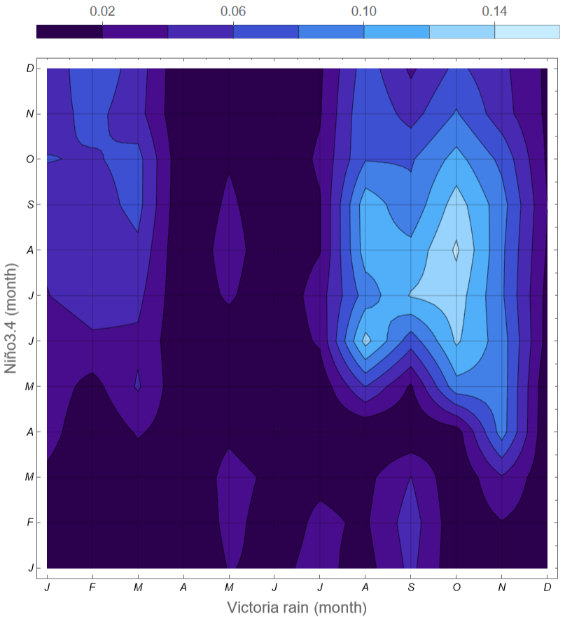
The plot indicates that Niño3.4 SSTs in July and August share information with the rainfall in October and to a lesser extent September. This is a highly useful relationship between a variable in wintertime and the rainfall in springtime.
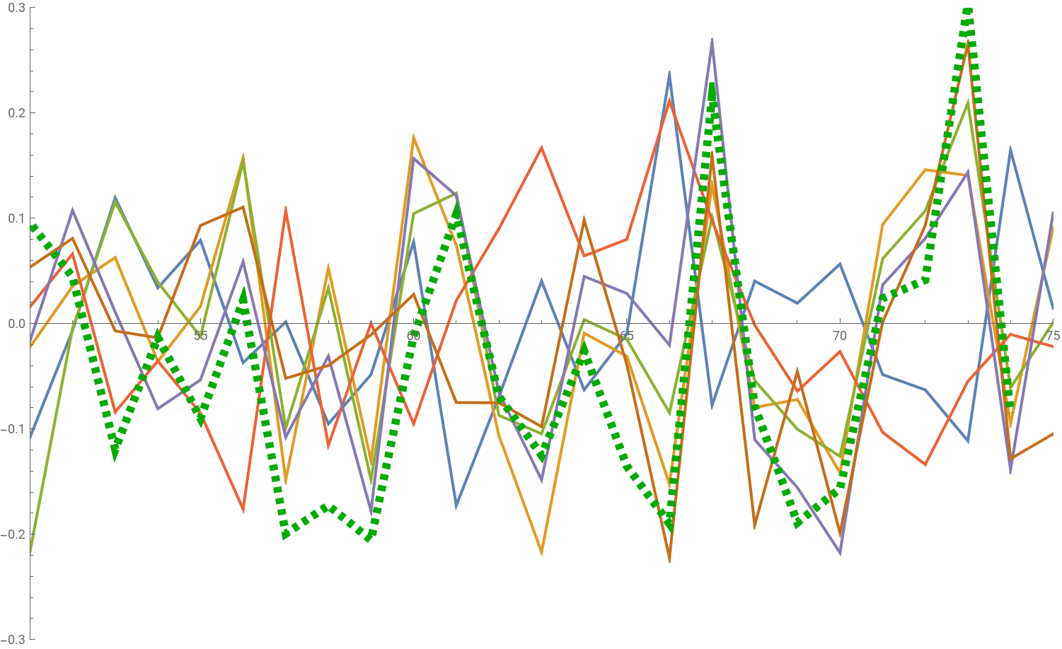
To illustrate the form of the input data we choose the task where at the end of July we wish to predict rainfall in SE Australia for the Sept/Oct period. Target rainfall over the 2000-2024 period is shown below as a green dotted line. Searching for variables that in July or earlier correlate with the future rainfall, we select the best six: Niño3.4 SST, Indian Ocean meridional gradients for June and July, SST at two positions in the Indian Ocean and the dominant principal component in the EOF expansion for Indian Ocean. The six (normalised) variables are shown in the plot below, where their (positive or negative) correlation with the rainfall is obvious but not a close match. The highest correlation is achieved by the EOF expansion, which matches two very wet years.
Neural network hind- and forecasting
Neural network hind- and forecasting
Next, we use the 24 years of data for the six variables as the input into a neural network. The data for each year are represented as a 6-vector. All variables except one are July sequences and all except Niño3.4 relate to the Indian Ocean. PC1 is the dominant principal component in the EOF expansion for the Indian Ocean sector 40E to 120E and 40S to 20N.
In[]:=
dim=6;InVect[j_]:={NinoJuly[[j]],.8MeridJuly[[j]],MeridJune[[j]],.8SIJuly[[j]],.8EIJuly[[j]],0.015PC1IndianJuly[[j]]};RainData=SESeptOctRainAnomaly;
Specify neural net and choose training parameters
In[]:=
net4=NetChain[{LinearLayer[dim],Tanh,LinearLayer[dim],LinearLayer[dim],LinearLayer[dim],LinearLayer[dim],LinearLayer[1]},"Input"->dim];StartYear=53;(*from1950,year2021is72*)StartValid=63;EndYear=74;ForecastEnd=75;(*Selecttraining,validationandforecastperiods*)Trials=20;(*Numberofrandomstarts*)Fc=True;(*Forecastattheendororhindcastforallyears*)LRateLow=.05;(*Networklearningratelowerlimit*)LRateHigh=.1;(*Networklearningratehigherlimit*)TrainingRounds=300;method="SignSGD";(*"ADAM"isalsoperformingwell*)frameLabel="SE Australia Sept/Oct Rainfall Anom. [mm]";yMin=-100;yMax=150;imageSize=700;
Next comes the training part, which is repeated many times (“Trials”) in order to accumulate the statistics on the dependence of the result on the learning rate (“LRate”) and get a measure of the errors. Learning rate is chosen as a random number between the low and high limits. Low learning rates lead to repeatable results, but not necessarily the best match. Higher learning rates result in large fluctuation of the results, and mostly the better match between their mean value and the desired outcome. With higher learning rates, over many trials the network configurations sample a number of local minima of the cost function and in most cases the mean is closer to the target.
The training, accumulating statistics and plotting of the result is performed by a separate module, attached to the post. The crucial part inside the module is a call to the very versatile NetTrain function, resulting in the trained network
DataInTrain=Table[InVect[j],{j,StartYear,StartValid-1}];DataInValid=Table[InVect[j],{j,StartValid,EndYear}];TrainGoal=Table[{RainData[[j]]},{j,StartYear,StartValid-1}];ValidGoal=Table[{RainData[[j]]},{j,StartValid,EndYear}];result4=NetTrain[net4,<|"Input"->DataInTrain,"Output"->TrainGoal|>,ValidationSet-><|"Input"->DataInValid,"Output"->ValidGoal|>,MaxTrainingRounds->TrainingRounds,Method->method,LearningRate->LearnRate];
Files required to run this example are attached. The example produces the following result
In this and all following plots, past measured rainfall anomaly is shown in green, separate training trials as faint grey lines and the average result during the validation period as a red line. The prediction for the current year using July data is shown in blue.
Skill of the method in hindcasting for the agriculturally important Murray-Darling area is lower, as shown in the examples below. On the left is the prediction with June data obtained using eight inputs, that include the Darwin and Tahiti sea level air pressures (components of the Southern Oscillation index). On the right, a prediction with July data uses only Niño3.4 SST and the first Indian Ocean EOF. The network was formed with data ending in the year 2020, and the following hindcasts (black) and a forecast (blue) are based on the 2020 network using new data. The agreement appears encouraging, but this is nevertheless mostly a hindcast. Occasional bad years, like 2013 in this example, can still occur.
November is more difficult to forecast, as the correlations between ocean indicators and the future rainfall are weaker. The example below was calculated in mid-September using the August data. In addition to the Nino3.4 and Indian Ocean gradient we use the information from the large Pacific area that correlates with November rainfall visible in the first figure. The input includes the second and third EOF for the area 140E to 100W and 40S to 5N and a gradient across the line dividing negative from positive correlation.
Overall, the predictions for 2024 do not provide important information about the skill of the method, as the rainfall is expected (also by the Australian Bureau of Meteorology) to be close to the average. The skill is best tested in forecasting large deviation years, like 2016 or 2022. This is more difficult, as shown for example by the failure [3] of the Bureau in 2020.
As weather phenomena are driven by the underlying chaotic dynamics, there is a limit to the predictability which depends on the form and the timescale of the applicable physical laws. To approach this limit, physical models and statistical models for medium term forecasting will need to converge as each method has different advantages. Improving the understanding between the ocean states and the future rainfall as attempted here is one of the many aspects of this fascinating problem.
As weather phenomena are driven by the underlying chaotic dynamics, there is a limit to the predictability which depends on the form and the timescale of the applicable physical laws. To approach this limit, physical models and statistical models for medium term forecasting will need to converge as each method has different advantages. Improving the understanding between the ocean states and the future rainfall as attempted here is one of the many aspects of this fascinating problem.
References
References
1. Bi, K. et al..: Accurate medium-range global weather forecasting with 3d neural networks. Nature, 619(7970), 1-6, doi:10.1038/s41586-023-06185-3, 2023.
2. Lam, R. et al.: Learning skilful medium-range global weather forecasting, Science 382, 1416-142, doi:10.1126/science.adi2336, 2023.
3. Lim, E. P. et al.: Why Australia was not wet during spring 2020 despite La Niña. Scientific Reports, 11, 18423, doi:10.1038/s41598-021-97690-w, 2021.
CITE THIS NOTEBOOK
CITE THIS NOTEBOOK
Forecasting seasonal rainfall in SE Australia using empirical orthogonal functions and neural networks
by Stjepan Marčelja
Wolfram Community, STAFF PICKS, September 25, 2024
https://community.wolfram.com/groups/-/m/t/3282530
by Stjepan Marčelja
Wolfram Community, STAFF PICKS, September 25, 2024
https://community.wolfram.com/groups/-/m/t/3282530