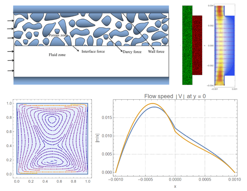
This project focuses on the development of computational models for a coupled flow scenario comprising of free and porous media. The fluid flow in the free region is governed by the Navier-Stokes PDE, while the flow in the porous region is governed by the Brinkman-Forchheimer PDE. A numerical solution for the coupled flow has been developed using the finite element method (FEM) framework in Wolfram Language, with conditional statements employed to enforce region-specific PDEs. An implicit issue with the continuity equation in the existing FluidFlowPDEComponent function was identified and resolved. In the latter part of the project, a custom function, BrinkmanPDEComponent, was developed in Wolfram Language to compute flow through porous media. The newly developed function supports both dimensional and non-dimensional forms of the Brinkman PDE. Detailed examples, scope, and applications of this new function are provided at the end of the post.
The project was conducted in collaboration with the numerics team at Wolfram Research. Special thanks to Stephen Wolfram for many helpful suggestions.
1. Introduction
1. Introduction
1.1. Real-world importance
1.1. Real-world importance
Solving coupled flow problems is crucial for many engineering applications. These problems arise in scenarios where different behaviors occur in each region, governed by distinct physical laws—such as the Navier-Stokes PDE for free flow and the Brinkman-Forchheimer PDE for porous media. Applications range from advanced heat sink and fuel cell designs to biological systems like transvascular fluid exchange [1-3]. Accurately capturing the transition of flow between the free and porous domains is essential for ensuring the performance and reliability of such systems.
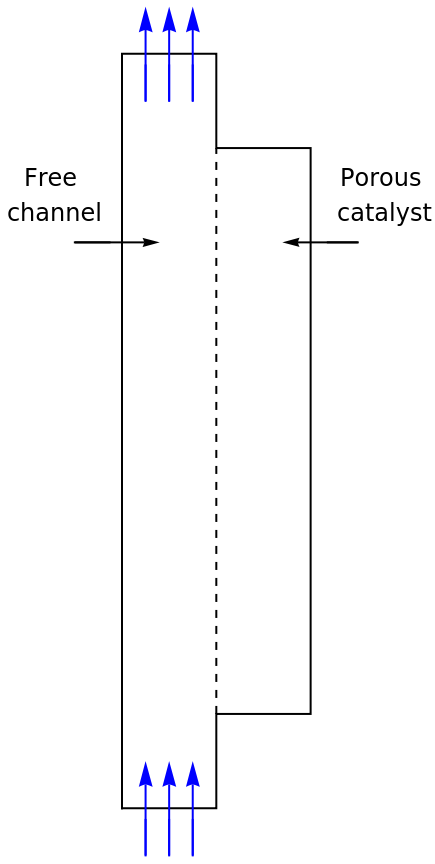
The model used in this project exemplifies fluid flow coupling between an open channel and a porous catalyst attached to one of the channel walls. The free flow is governed by the Navier-Stokes PDE, while the porous region is governed by the Brinkman-Forchheimer PDE. The project draws on the work of Amiri and Vafai [4] and the Forchheimer Flow documentation of COMSOL [5].
The model used in this project exemplifies fluid flow coupling between an open channel and a porous catalyst attached to one of the channel walls. The free flow is governed by the Navier-Stokes PDE, while the porous region is governed by the Brinkman-Forchheimer PDE. The project draws on the work of Amiri and Vafai [4] and the Forchheimer Flow documentation of COMSOL [5].
1.2. Objectives of the Post
1.2. Objectives of the Post
This post demonstrates advanced techniques for modeling coupled free and porous media flows using Wolfram Language. The key goals include:
◼
Developing a computational model that accurately solves coupled flow in dual-region domains, where free flow governed by the Navier-Stokes PDE transitions into porous flow governed by the Brinkman-Forchheimer PDE.
◼
Highlighting the use of the FluidFlowPDEComponent function in Wolfram Language to handle the Navier-Stokes part in coupled flow.
◼
Introducing the custom function BrinkmanPDEComponent for modeling porous media flow in both dimensional and non-dimensional forms.
2. Setting up the Finite Element Mesh
2. Setting up the Finite Element Mesh
2.1. Computational Domain
2.1. Computational Domain
In this project, we model the fluid flow through a dual-region channel consisting of a free-flow region and a porous catalyst. Evaluating the following code gives us a schematic
of this computational domain.
of this computational domain.
In[154]:=
schematic=Graphics[]
Out[154]=
2.2. Defining Regions and Mesh
2.2. Defining Regions and Mesh
To begin, we need to create a mesh that represents the computational domain. To define this mesh, We will need the ToBoundaryMesh and ToElementMesh functions from finite element method (FEM) package of Wolfram Language.
First, load the necessary package that contains the finite element method tools:
In[155]:=
Needs["NDSolve`FEM`"];
Evaluating the above statement loads the finite element method package, providing access to the required tools for mesh generation.
2.3. Defining Coordinates and Connectivity
2.3. Defining Coordinates and Connectivity
Next, we define the coordinates of the points that make up our mesh and specify how these points are connected.
The coordinates variable stores the positions of the nodes in our domain:
In[156]:=
coordinates={{-,-},{0,-},{0,-},{,-},{,},{0,},{0,},{-,}};
1
3
10
4
3
10
4
3
10
3
3
10
1
3
10
3
3
10
1
3
10
3
3
10
3
3
10
4
3
10
1
3
10
4
3
10
The connectivity variable defines how these nodes are linked to form the boundary elements:
In[157]:=
connectivity=LineElement[{{1,2},{2,3},{3,4},{4,5},{5,6},{6,7},{7,8},{8,1},{3,6}}];
We now create the boundary mesh bmesh using the ToBoundaryMesh function. The boundary mesh defines the outer boundary of the problem domain.
In[158]:=
bmesh=ToBoundaryMesh["Coordinates"coordinates,"BoundaryElements"connectivity];
Note that the coordinates and connectivity previously defined are passed into this function to form the boundary elements.
Next, we define two points, one inside the free-flow region and one inside the porous region. We call each of these points a RegionMarker. These points will act as markers that help us specify the regions where the respective PDEs should be applied.
In[159]:=
freeCoordinate={-5*,0};
-4
10
In[160]:=
porousCoordinate={5*,0};
-4
10
Note that freeCoordinate is an arbitrary point located in the free-flow region, and porousCoordinate is an arbitrary point located in the porous region.
Next, we generate the computational mesh mesh using the ToElementMesh function. This converts the boundary mesh into a mesh suitable for finite element analysis.
In[161]:=
mesh=ToElementMesh[bmesh,"RegionMarker"->{{freeCoordinate,1},{porousCoordinate,2}},"MaxCellMeasure"{"Length"2*}];
-4
10
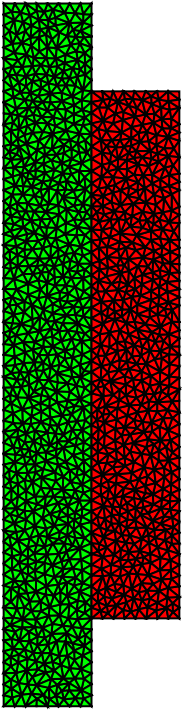
Note here that the RegionMarker option maps the freeCoordinate to region 1 and the porousCoordinate to region 2. The MaxCellMeasure option refines the mesh by controlling the maximum cell size, improving accuracy during finite element analysis.
Let’s visualize the mesh that we have created by evaluating the following statement:
In[162]:=
mesh["Wireframe"["MeshElementStyle"{Directive[FaceForm[Green]],Directive[FaceForm[Red]]}]]
Out[162]=
Now that we have started working with the computational domain, in this section we digress briefly from the computational setup to understand the flow PDEs governing our model.
The flow is governed by two distinct physical laws:
◼
The Navier-Stokes PDE for the free flow region, and
◼
The Brinkman-Forchheimer PDE for the porous region.
The Navier-Stokes PDEs are used to model the fluid flow in the free channel, and they are given by:
The Brinkman-Forchheimer PDEs are used to model the fluid flow in the porous region, and they are given by:
3.2. Brief note on the need for Brinkman’s Extension to Darcy’s Law
3.2. Brief note on the need for Brinkman’s Extension to Darcy’s Law
It is known that Darcy’s law governs the fluid flow in a porous region, assuming a linear relationship between the pressure gradient ∇p and the volumetric flux V [6]. Darcy’s law is given by the equation:
Darcy’s law works well for laminar flows at low Reynolds numbers where assumption of linearity holds. However, as velocity increases, viscous shear effects become significant, meaning the linear assumption no longer holds, and a modification is needed for higher velocity flows.
3.2.1. Brinkman’s contribution
3.2.1. Brinkman’s contribution
Henry Coenraad Brinkman, in his work from 1949 [7] studied this issue about limitation of Darcy’s law to laminar flows at low Reynolds numbers. He looked at the Darcy’s law and compared it with a form of Navier-Stokes equation where viscous terms dominate over inertial terms:
where μ’ (viscosity in the shear term) accounts for viscous shear effects.
Brinkman proposed modifying Darcy’s law to include the viscous shear effects by combining it with the form of the Navier-Stokes equation where viscous terms dominate over inertial terms. This modification leads to the formulation better suited for higher velocities and able to handle boundary conditions more effectively.
Now we will set up the coupled flow model using the region markers that we defined earlier. These markers allow us to assign different PDE coefficients to respective regions. The conditional statements in the model use the ElementMarker approach to determine whether the flow is in the free-flow or porous region and apply the appropriate PDE for each.
We define the nonhomogeneous part of the Brinkman-Forchheimer PDE (Forchheimer term) as follows:
Note that to make sure that the Forchheimer term only applies to the Brinkman-Forchheimer PDE, we again use the conditional statements along with ElementMarker.
We now define the parameters for our coupled model:
At the remaining boundaries the flow velocity V is set to 0 to model the solid walls where the fluid has no-slip.
Finally, we group all the boundary conditions into a list bcs that we can use
We begin by solving the flow model without the Forchheimer correction term to observe how the flow behaves under this simplified condition.
The following code sets up the fluid dynamics PDE model without the Forchheimer correction term F:
◼
The function NDSolveValue numerically solves differential equations and returns interpolating functions for the specified variables—in this case, u, v, and p—over the computational domain.
◼
The solutions will be stored in ufun, vfun, and pfun. They are functions (more specifically, interpolating functions) that represent the numerical solutions for the variables u, v, and p respectively.
◼
InitialSeeding sets the initial conditions or initial guesses for the solver to start the numerical computation. Setting the initial values can help improve convergence and computational efficiency. We set :
◼
u[x, y] == 0, which means the initial horizontal velocity is zero
◼
p[x, y] == 0, which means the initial pressure is zero
◼
The following code sets up the PDE model with the Forchheimer correction term F:
Note that this time, the solution is stored in ufunCorrected, vfunCorrected, and pfunCorrected. Note further that we use the existing solution for the initial seeding (from ufun, vfun, and pfun) to provide a good initial guess for the solver and help in convergence.
It’s time to visualize the results!
We start by visualizing the velocity field across the channel. The side-by-side plots below show how the flow behaves without and with the Forchheimer correction.
We have the contour plots! We note that there are slight differences in the plots with and without Forchheimer term. Thus, to visualize better, we zoom in on the flow speed by plotting it along the middle of the channel (y = 0).
This comparison helps to highlight the differences between the corrected and uncorrected flows. These results are consistent with the result from COMSOL documentation [5] .
In the previous section, we constructed the free flow part of the coupled model by manually writing the Navier-Stokes PDE into our model. Instead of having to manually write down the PDEs, we can also use a relevant component from the PDE component library of Wolfram Language. We will use FluidFlowPDEComponent from this library to build a more compact and efficient model of our system.
The first step is comparing the coefficients of the Navier-Stokes momentum PDE with the coefficients of the Brinkman-Forchheimer PDEs to identify the differences and modifications required:
We note that:
◼
The Navier-Stokes momentum PDE has terms for density (ρ) and dynamic viscosity (μ).
◼
The Brinkman-Forchheimer PDE includes modified terms for permeability (κ) and porosity (ϕ).
Thus, FluidFlowPDEComponent can be used to solve the Navier-Stokes part by modifying it in the following way:
1
.Making the following replacements in the function parameters for region 2:
1
.1
.Replacing the mass density ρ with 0.
Making the aforementioned modifications in the FluidFlowPDEComponent gives the following flow model:
The parameters and boundary conditions for the model have been defined earlier and will be passed down to the present model. Thus we directly move on to solving the PDEs in the next section.
As earlier, we begin by solving the flow model without the Forchheimer correction term first. The following code sets up the fluid dynamics PDE model without the Forchheimer correction term F:
Here, we have encountered an error in the solution! What it might be?
If we note the coupledFlowModel that we just created, we will realize that the continuity equation in the free-flow region would become an identity. This can be corrected by replacing the third component in coupledFlowModel with ∇·V, which can be done as follows:
The ∇·V expression will now result in the equation ∇·V = 0 instead of 0 = 0 in the definition of the coupled flow PDE, which we set again as follows:
We now set up the PDE model with the Forchheimer correction term F:
We visualize the results similarly as in section 4. The plots below show how the flow behaves without and with the Forchheimer term:
To visualize better, we plot the flow speed along the middle of the channel (y = 0):
These results are consistent with our previous results and the COMSOL documentation [5].
Unlike FluidFlowPDEComponent, which is a built-in function in Wolfram Language that generates the PDE component for the Navier-Stokes PDE, there isn't a similar built-in function yet for the Brinkman PDE. So, let' s create that function ourselves.
The present section briefly illustrates how such a function might be created. The BrinkmanPDEComponent that we create below handles both the dimensional and non - dimensional forms of the Brinkman PDE.
BrinkmanPDEComponent returns a sum of differential operators to be used in PDEs and can handle both dimensional and non-dimensional forms of the Brinkman PDE. Detailed examples, scope, and applications of this function are provided in this section as well.
The equation of the model BrinkmanPDEComponent with dynamic viscosity μ, porosity ϕ, and permeability κ is based on the Brinkman’s momentum PDE and the continuity equation:
The following sections present a preliminary documentation for the BrinkmanPDEComponent, which has been submitted to the Wolfram Function Repository:
The BrinkmanPDEComponent[vars,pars] function provides the symbolic structure of the Brinkman’s equation for porous media flow. This function can take one of two sets of parameters:
◼
Dynamic Viscosity, Porosity, and Permeability, or
◼
Reynolds Number and Darcy Number.
The function is defined as follows :
◼
BrinkmanPDEComponent models the flow of viscous fluids through porous media under applied constraints.
◼
BrinkmanPDEComponent returns a sum of differential operators to be used as a part of partial differential equations:
◼
BrinkmanPDEComponent creates PDE components for stationary parametric analysis.
◼
BrinkmanPDEComponent creates PDE components in two and three space dimensions
◼
BrinkmanPDEComponent creates a system of equations with the vector-valued Brinkman’s momentum equation combined with the continuity equation.
◼
The following parameters pars can be given:
Define flow PDE through a porous medium:
Specify a symbolic stationary flow PDE through porous medium in two dimensions with dynamic viscosity μ, porosity ϕ, and permeability κ:
Specify a symbolic stationary flow PDE through porous medium in three dimensions with dynamic viscosity μ, porosity ϕ, and permeability κ:
Solve for the velocity and pressure in a porous cavity with antiparallel flow and a source term:
Visualize the velocity of the fluid:
1
.Coupled FluidFlowPDEComponent with the Brinkman’s PDE to develop the flow model for a coupled free and porous media flow.
◼
Identified an issue where defining the continuity equation explicitly in its reduced form is necessary; otherwise, it causes the continuity equation to become an identity in region 2.
2
.Developed the BrinkmanPDEComponent function for the 2D and 3D cases of Brinkman’s PDEs which govern porous media flows with high Reynolds numbers with significant viscous shear effects.
◼
The newly developed function accepts:
◼
Dynamic viscosity, porosity, and permeability (for dimensional form of the PDE)
◼
Reynolds number and Darcy number (for non-dimensional form of the PDE)
◼
Preliminary documentation includes:
◼
Test-cases and examples
◼
Scope of the function
◼
Application
The project involved development of computational models for solving PDEs in coupled flow with free and porous regions. The free flow is governed by the Navier-Stokes PDEs and the porous region is governed by Brinkman-Forchheimer PDEs.
First, the FluidFlowPDEComponent was successfully implemented to solve the Navier - Stokes PDEs in the free - flow region of the computational domain . Defining the continuity equation explicitly in its reduced form was necessary, and without this adjustment, the continuity equation would become an identity and cause errors in the model.
Secondly, a custom function BrinkmanPDEComponent was developed to handle porous media flow with high Reynolds numbers and significant viscous shear effects. This newly developed function accommodates both dimensional and non-dimensional forms of the Brinkman PDEs.
Finally, preliminary documentation and basic examples were provided to demonstrate the functionality of the new component, which successfully models flow in 2D and 3D porous media.
My deepest gratitude goes to Sotiris for his invaluable support, and to John for his assistance in the planning and execution of this project.
Special thanks to Stephen Wolfram for his encouragement and insightful discussions on the fluid flow equations that form the core of this work.
I am grateful to Oliver Rübenkönig and the numerics team at Wolfram Research for providing a project that was both challenging and rewarding. Thanks to Mads and his team for making the Wolfram Summer School an invaluable experience.
Finally, my heartfelt thanks to my wife and family for their unwavering love and support, especially through the birth of our daughter during the summer school .
References
References
1
.McCurdy, M. et al. (2019)Convection in a coupled fluid-porous media system. arXiv, 1901.02925. https://doi.org/10.48550/arXiv.1901.02925
2
.Baber, K. I. (2014). Coupling free flow and flow in porous media in biological and technical applications: From a simple to a complex interface description (Doctoral dissertation). University of Stuttgart, Stuttgart, Germany.
3
.Waghode, A. N. (2005). Computational fluid dynamics of coupled free/porous regimes: A specialised case of pleated cartridge filter (Master’s thesis). Loughborough University. https://dspace.lboro.ac.uk/2134/35467
4
.Amiri, A., & Vafai, K. (1998). Transient analysis of incompressible flow through a packed bed. International Journal of Heat and Mass Transfer, 41(24), 4259-4279. https://doi.org/10.1016/S0017-9310(98)00120-3
5
.Forchheimer Flow. COMSOL Multiphysics 5.5 Documentation. Retrieved October 17, 2024, from www.comsol.com/model/download/656391/models.porous.forchheimer_flow.pdf
6
.Whitaker, S. (1986). Flow in porous media I: A theoretical derivation of Darcy’s law. Transport in Porous Media, 1, 3–25. https://doi.org/10.1007/BF01036523
7
.Brinkman, H. C. (1949). A calculation of the viscous force exerted by a flowing fluid on a dense swarm of particles. Applied Scientific Research, 1, 27–34. https://doi.org/10.1007/BF02120313
8
.Image credit : Li, Z . et al . (2018) . "Implementation and verification of finite volume compressible solver for porous-fluid coupling problem," International Journal of Heat and Mass Transfer.
Access the Full Code
Access the Full Code
Cite This Notebook
Cite This Notebook
Solving Navier-Stokes and Brinkman-Forchheimer PDEs for Coupled Free and Porous Media Flow
by Safi Ahmed
Wolfram Community, STAFF PICKS, July 11, 2024
https://community.wolfram.com/groups/-/m/t/3210114
by Safi Ahmed
Wolfram Community, STAFF PICKS, July 11, 2024
https://community.wolfram.com/groups/-/m/t/3210114