Wolfram Cloud Document

A data set on the prevalence of infection for an outbreak lasting 200 days in a population of 500 people is given, as shown in the table below .

In[]:=

Clear["Global`*"]

data={{10,19},{17,4},{24,5},{32,47},{36,38},{38,54},{41,84},{42,55},{47,116},{50,102},{52,126},{58,153},{59,164},{62,172},{63,177},{67,142},{68,158},{69,151},{75,155},{80,125},{81,116},{84,101},{87,106},{88,116},{94,85},{98,59},{102,67},{105,57},{114,59},{117,24},{118,39},{120,31},{128,36},{134,8},{140,7},{142,3},{147,20},{150,7},{155,2},{159,25},{163,2},{186,10},{191,17},{200,7}};dataTable=TableForm[data,TableHeadings->{None,{"Time","Number Infected"}}]

Out[]//TableForm=

Time	Number Infected
10	19
17	4
24	5
32	47
36	38
38	54
41	84
42	55
47	116
50	102
52	126
58	153
59	164
62	172
63	177
67	142
68	158
69	151
75	155
80	125
81	116
84	101
87	106
88	116
94	85
98	59
102	67
105	57
114	59
117	24
118	39
120	31
128	36
134	8
140	7
142	3
147	20
150	7
155	2
159	25
163	2
186	10
191	17
200	7

pointsPlot=ListPlot[data,PlotStyle->PointSize[Medium],Frame->True,FrameLabel->{"Time (days)","Number Infected"},GridLines->Automatic,GridLinesStyle->LightGray,PlotRange->{{0,210},{-5,350}},BaseStyle->{FontSize->14},ImageSize->400]

Out[]=

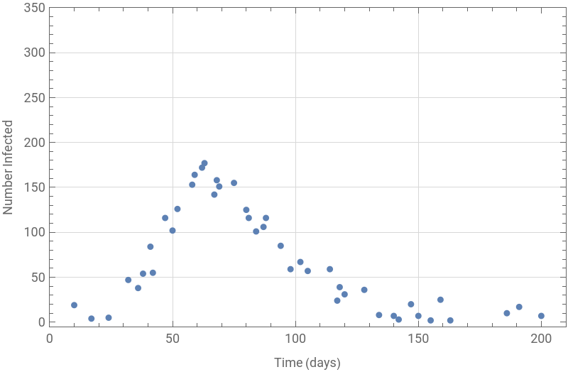
Plotting the dataset, this look like an epidemic curve for an outbreak starting with the introduction of one infected case . We have data points of the prevalence of infection spanning the entire duration of the epidemic (200 days), but not for every day . Define the simple SIR model and model input:

What are the best - fitting values for
β
and
γ
?

In[]:=

(*totalsizeofpopulation*)n=500;

In[]:=

times=data[[All,1]]

Out[]=

{10,17,24,32,36,38,41,42,47,50,52,58,59,62,63,67,68,69,75,80,81,84,87,88,94,98,102,105,114,117,118,120,128,134,140,142,147,150,155,159,163,186,191,200}

In[]:=

(*Fludataset*)numberinfected=data[[All,2]]

Out[]=

{19,4,5,47,38,54,84,55,116,102,126,153,164,172,177,142,158,151,155,125,116,101,106,116,85,59,67,57,59,24,39,31,36,8,7,3,20,7,2,25,2,10,17,7}

In[]:=

ClearAll[β,γ]sireqns={s'[t]==-β*s[t]*i[t]/n,i'[t]==β*s[t]*i[t]/n-γ*i[t],r'[t]==γ*i[t]};initialConditions={s[0]==n,i[0]==1,r[0]==0};

In[]:=

sol=ParametricNDSolve[{sireqns,initialConditions},{s,i,r},{t,0,times},{β,γ}];

In[]:=

(*Extracttheinfectedvaluesfromthesolution*)infectedValues=i/.sol;

objective[b_,g_]:=Norm[(infectedValues[b,g][times]-numberinfected)]^2bDom=Range[0,2,0.01];gDom=Range[0,1,0.01];res=Flatten[Table[{b,g,objective[b,g]},{b,bDom},{g,gDom}],1];Flatten[res[[PositionSmallest[res[[All,3]]]]]]//Most

Out[]=

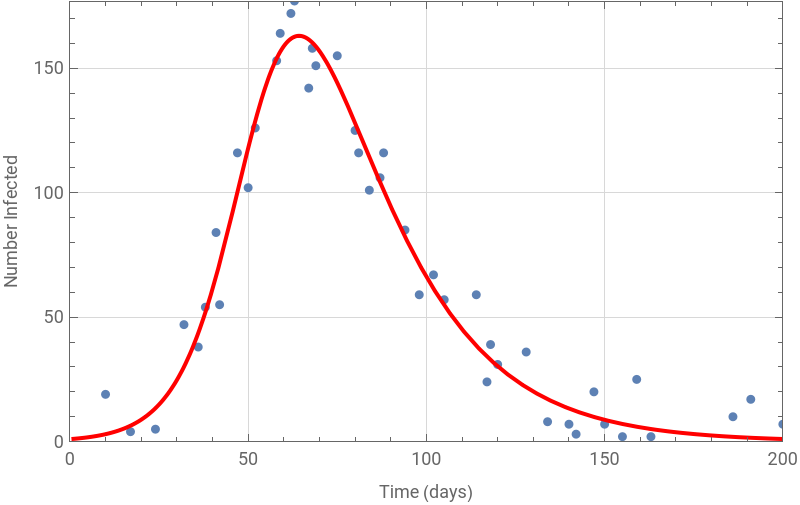
{0.16,0.05}

We can confirm visually that this parameter set produces a good model fit to the data, by overlaying the datapoints on a plot of the model output:

(*Setparametervalues*){β,γ}={0.16,0.05};(*DefinetheSIRmodelequations*)sireqns={s'[t]==-β*s[t]*i[t]/n,i'[t]==β*s[t]*i[t]/n-γ*i[t],r'[t]==γ*i[t]};initialConditions={s[0]==n,i[0]==1,r[0]==0};

(*Solvethedifferentialequations*)sol=NDSolve[{sireqns,initialConditions},{s,i,r},{t,0,times}];

In[]:=

(*Extracttheinfectedvaluesfromthesolution*)infectedValues=i/.sol[[1]];

In[]:=

(*Calculatethesum-of-squares(SSQ)value*)ssq=Norm[infectedValues[Range[times]]-numberinfected]^2;

Norm

:The first Norm argument should be a scalar, vector, or matrix.

fitPlot=Plot[infectedValues[t],{t,1,200},PlotStyle->Red];Show[pointsPlot,fitPlot,PlotRange->All]

Out[]=

Based on our estimates parameter values, what would be the critical vaccination threshold required to prevent this epidemic, assuming an all - or - nothing vaccine with 75 % efficacy?

We can calculate the critical effective vaccination coverage as :

eff

1-

0.05

0.16

0.69

Since the all - or - nothing vaccine is only 75 % effective, we can calculate the critical vaccination threshold as :



eff



0.69

0.75

0.92

To interrupt transmission and bring

, 92 % of the population would have to be vaccinated . We can confirm the absence of an epidemic under these conditions using the simulation code :

In[]:=

(*only8%ofthepopulationaresusceptible,92%ofthepopulationarevaccinated/immune*)initialConditionsvac={s[0]==499*0.08,i[0]==1,r[0]==499*0.92};

sol1=NDSolve[{sireqns,initialConditionsvac},{s,i,r},{t,0,200}];

CITE THIS NOTEBOOK

Optimizing transmission & recovery parameters to fit flu infection data in a calibrated SIR model
by Athanasios Paraskevopoulos
Wolfram Community, STAFF PICKS, August 29, 2023
https://community.wolfram.com/groups/-/m/t/3000833

What are the best - fitting values for β and γ?

CITE THIS NOTEBOOK

What are the best - fitting values for
β
and
γ
?