The following research, which is part of my thesis and is based on “Dynamics of nonlinear lattices: asymptotic behavior and study of the existence and stability of tracked oscillations,” investigates what happens when the position and velocity at the boundary points must be prescribed. Therefore, I chose to set both the position and velocity to zero at both endpoints.
The study of the dynamics of the discrete Klein - Gordon equation (DKG) with friction is given by the equation : -K(-2+)+δ+()0; β>0,δ>0In the above equation, describes the potential function :
̈
U
n
U
n+1
U
n
U
n-1
U
n
′
W
U
n
W
W()-+
U
n
2
w
d
2
2
U
n
β
2
w
d
4
4
U
n
The objective of this simulation is to model the dynamics of a segment of DNA under thermal fluctuations with fixed boundaries using a modified discrete Klein-Gordon equation. The model incorporates elasticity, nonlinearity, and damping to provide insights into the mechanical behavior of DNA under various conditions.
In[]:=
(*AdjustedParameters*)numBases=200;(*Numberofbasepairs,representingasegmentofDNA*)kappa=0.1;(*Elasticityconstant,chosentoreflectthestiffness;arbitraryunit*)omegaD=0.2;(*Frequencyterm,speculativeandlowtoreflectslowdynamics*)beta=0.05;(*Nonlinearitycoefficientsmalltointroducemildnonlinearity*)(*Dampingcoefficient*)delta=0.01;
◼
Position: Random initial perturbations between 0.01 and 0.02 to simulate the thermal fluctuations at the start.
◼
Velocity: All bases start from rest, assuming no initial movement except for the thermal perturbations.
(*Introducingrandominitialperturbationstosimulatethermalfluctuations*)initialPositions=Table[x[n][0]==RandomReal[{0.01,0.02}],{n,1,numBases}];initialVelocities=Table[x[n]'[0]==0,{n,1,numBases}];(*Assuminginitialreststate*)
The simulation uses fixed ends to model the DNA segment being anchored at both ends, which is typical in experimental setups for studying DNA mechanics.
(*BoundaryConditions*)(*FixedendstosimulateasegmentofDNAanchoredatbothends*)boundaryConditions={x[0][t]==0,x[numBases+1][t]==0};
The equations of motion for each base are derived from a modified discrete Klein-Gordon equation with the inclusion of damping:
(*Equations*)equations=Table[x[n]''[t]-kappa(x[n+1][t]-2x[n][t]+x[n-1][t])+deltax[n]'[t]+omegaD^2(x[n][t]-betax[n][t]^3)==0,{n,1,numBases}];(*SolveNumerically*)solution=NDSolveValue[{equations,initialPositions,initialVelocities,boundaryConditions},Table[x[n],{n,1,numBases}],{t,0,50}];
(*Visualization*)Plot[Evaluate[Table[solution[[n]][t],{n,1,numBases}]],{t,0,50},PlotLegends->Table[StringJoin["Base ",ToString[n]],{n,1,numBases}],PlotRange->All]
Out[]=

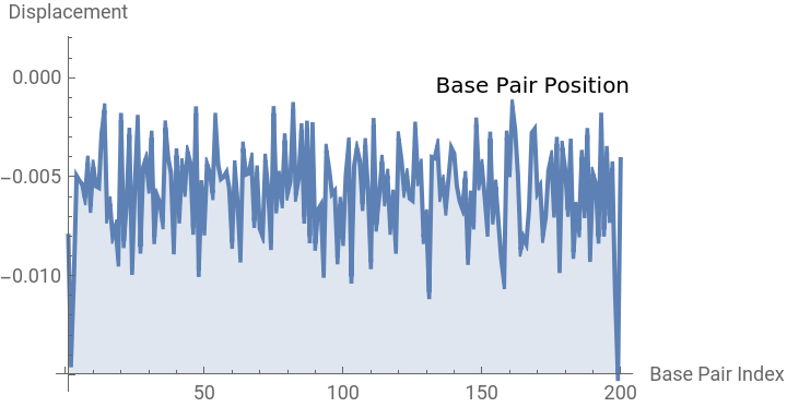
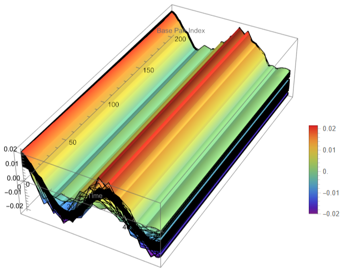
The results are visualized using a plot that shows the displacements of each base over time . Key observations from the simulation include :
◼
Wave Propagation: The initial perturbations lead to wave-like dynamics along the segment, with visible propagation and reflection at the boundaries.
◼
Damping Effects: The inclusion of damping leads to a gradual reduction in the amplitude of the oscillations, indicating energy dissipation over time.
◼
Nonlinear Behavior: The nonlinear term influences the response, potentially stabilizing the system against large displacements or leading to complex dynamic patterns.
In[]:=
(*Chooseaspecifictimeforthesnapshot*)snapshotTime=10;(*GenerateDiscretePlotfortheDNAmodelatthesnapshottime*)DiscretePlot[solution[[n]][snapshotTime],{n,1,numBases},PlotRange->All,PlotStyle->PointSize[Medium],PlotLabels->Placed["Base Pair Position",Above],AxesLabel->{"Base Pair Index","Displacement"}]

Out[]=
In[]:=
(*3DVisualization*)Plot3D[Evaluate[Table[solution[[n]][t],{n,1,numBases}]],{t,0,50},{n,1,numBases},AxesLabel->{"Time","Base Pair Index","Displacement"},PlotRange->All,Mesh->None,ColorFunction->"Rainbow",PlotLegends->Automatic,AxesOrigin->{0,1,0},BoxRatios->{1,2,0.5}]
In[]:=
(*3DVisualization*)data=Table[solution[[n]][t],{n,1,numBases},{t,0,50,1}];ListPlot3D[data,Mesh->None,AxesLabel->{"Base Pair","Time","Displacement"},PlotLabel->"Dynamics of DNA Segment",PlotRange->All,ColorFunction->"Rainbow"]
Out[]=

(*Generatedatafor3Dplot*)data=Flatten[Table[{n,t,solution[[n]][t]},{n,1,numBases},{t,0,50,0.5}],1];(*3DPlot*)ListPointPlot3D[data,AxesLabel->{"Base Pair","Time","Displacement"},PlotRange->All,ColorFunction->"Rainbow",PlotStyle->PointSize[Small]]

(*Choosespecifictimepointsforvisualization*)timePoints={0,10,20,30,40,50};(*Generatedataforeachtimepoint*)dataAtTimePoints=Table[Table[{n,time,solution[[n]][time]},{n,1,numBases}],{time,timePoints}];(*3DDiscretePlot*)Graphics3D[{Table[{Hue[time/Max[timePoints]],PointSize[0.02],Point[data]},{time,timePoints},{data,dataAtTimePoints[[Position[timePoints,time][[1,1]]]]}]},Axes->True,AxesLabel->{"Base Pair","Time","Displacement"},BoxRatios->{1,1,0.5},PlotRange->All]
Out[]=

In[]:=
(*Generatedatafor3Dplotefficiently*)If[ListQ[solution],data=ParallelTable[{n,t,solution[[n]][t]},{n,1,numBases},{t,0,50,0.5}],MessageDialog["Solution is not available. Check the differential equation solver outputs."]];(*Moreefficientflattening*)data=Flatten[data,1];(*Enhanced3DVisualizationwithSurfacePlot*)ListPlot3D[data,AxesLabel->{"Base Pair","Time","Displacement"},PlotRange->All,ColorFunction->"TemperatureMap",Mesh->None,PlotTheme->"Detailed",BoxRatios->{1,2,0.5}](*Addinginteractivity*)Manipulate[ListPlot3D[Select[data,#[[2]]<=time&],AxesLabel->{"Base Pair","Time","Displacement"},PlotRange->{{1,numBases},{0,time},All},ColorFunction->"TemperatureMap",Mesh->None,PlotTheme->"Detailed",BoxRatios->{1,2,0.5}],{time,0,50,0.5,Appearance->"Labeled"}]
Stationary points in this context refer to positions where the rate of change of displacement (both velocity and acceleration) approaches zero, indicating points of equilibrium or stable configurations under certain conditions.
CITE THIS NOTEBOOK
CITE THIS NOTEBOOK
Exploring the effects of non-linearity and damping on DNA base pair dynamics through simulation
by Athanasios Paraskevopoulos
Wolfram Community, STAFF PICKS, May 5, 2024
https://community.wolfram.com/groups/-/m/t/3170456
by Athanasios Paraskevopoulos
Wolfram Community, STAFF PICKS, May 5, 2024
https://community.wolfram.com/groups/-/m/t/3170456