This computational essay studies binary error-correcting codes as finite sphere packings inside Hamming space. A binary word is a vertex of the cube {0,1}^n, and a code is a selected set of vertices. The central question is whether direct random accretion can approach the performance of structured Hamming and Golay codes. The experiments compare code sizes to a common finite bound and report both average and best random performance. In the small Hamming case, the best random trial can sometimes match the structured size, but the typical random construction is less reliable. At larger distances and Golay-scale parameters, algebraic structure remains far stronger than direct random search.
Introduction
Introduction
History and Nomenclature
History and Nomenclature
A code is a set C of allowed messages, called codewords, chosen from a larger space of possible words. In this essay the words are binary strings, so C is a subset of {0,1}^n. Error-correcting codes began in the late 1940s after Claude Shannon showed that reliable communication is possible even through noisy channels, as long as information is encoded with enough redundancy. Richard Hamming then created the first practical Hamming codes after becoming frustrated with errors in early computers.
A perfect code is a code that packs Hamming spheres so efficiently that every possible received word lies within exactly one correction sphere around a valid codeword. Hamming codes are the classic perfect 1-error-correcting codes, such as the binary [7,4,3] Hamming code. The binary [23,12,7] Golay code is another rare perfect code and corrects up to 3 errors.
In the notation [n,k,d], n is the block length, k is the number of information bits, and d is the minimum Hamming distance between two distinct codewords. Since k information bits have 2^k possible messages, a binary [n,k,d] linear code contains 2^k codewords.
Hamming Space as a Discrete Geometry
Hamming Space as a Discrete Geometry
A binary word of length n is a vertex of the cube {0,1}^n. The Hamming distance d_H(x,y) counts how many coordinates differ. Thus, distance is not a metaphor but rather the graph distance in the n-dimensional cube. A binary code C is a selected subset of these vertices.
d_H(x,y) = |{i : x_i ≠ y_i}|
The minimum distance d(C) is the smallest distance between two distinct codewords. If d(C) is large, then codewords are separated by many bit flips, and small error balls around codewords do not overlap.
The minimum distance of a code is the smallest Hamming distance between two distinct codewords. This definition uses unordered pairs, so the diagonal of the distance matrix is never considered:
In[]:=
ClearAll[minHammingDistance];minHammingDistance[code_]:=Min[Select[Flatten[DistanceMatrix[code,DistanceFunction->HammingDistance]],Positive]]
In[]:=
Grid[{{"calculation","value"},{"HammingDistance[{1,0,0},{0,1,0}]",HammingDistance[{1,0,0},{0,1,0}]},{"minHammingDistance[{{0,0,0},{1,1,0},{1,1,1}}]",minHammingDistance[{{0,0,0},{1,1,0},{1,1,1}}]}},Frame->All]
Out[]=
calculation | value |
HammingDistance[{1,0,0},{0,1,0}] | 2 |
minHammingDistance[{{0,0,0},{1,1,0},{1,1,1}}] | 1 |
In[]:=
"calculation" | "value" |
"HammingDistance[{1,0,0},{0,1,0}]" | 2 |
"minHammingDistance[{{0,0,0},{1,1,0},{1,1,1}}]" | 1 |
Out[]=
calculation | value |
HammingDistance[{1,0,0},{0,1,0}] | 2 |
minHammingDistance[{{0,0,0},{1,1,0},{1,1,1}}] | 1 |
The first distance is 2 because the two words differ in two coordinate positions. The small three-word code has minimum distance 1 because two of its words differ in only one coordinate.
The 3-Cube
The 3-Cube
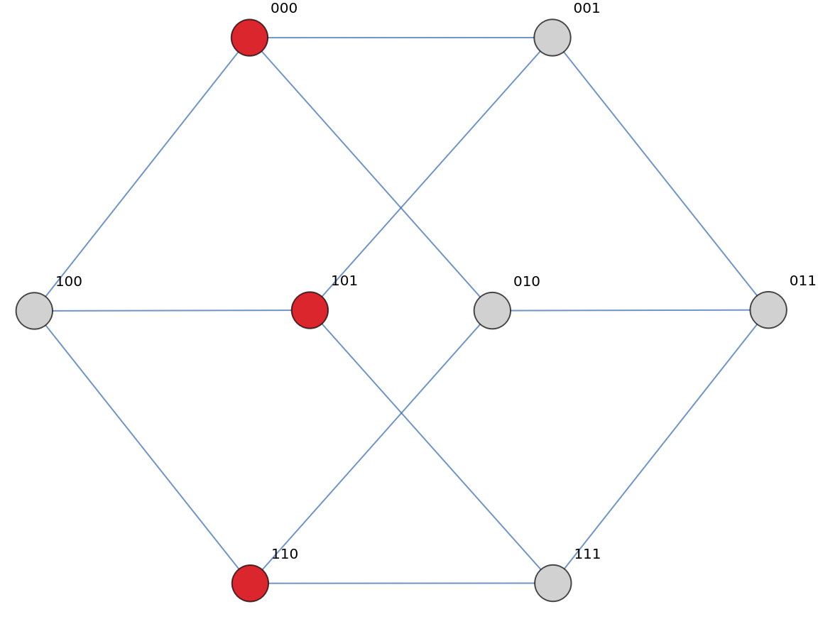
The 3-dimensional cube gives a concrete picture of Hamming space. Edges connect words at distance 1.
The function cubeWord converts a vertex index into the corresponding binary word in {0,1}^n. The two-argument form is used so the dimension and index are always visible at the call site:
In[]:=
ClearAll[cubeWord];cubeWord[n_Integer,i_Integer]:=IntegerDigits[i-1,2,n]
cubeIndex[v_List] converts a binary word into the corresponding cube vertex index:
In[]:=
ClearAll[cubeIndex]cubeIndex[v_List]:=FromDigits[v,2]+1
For larger generated codes, literal cube drawings stop being useful. The notebook therefore switches to distance matrices, histograms of random trial outcomes, and percentages relative to the Hamming bound. These summaries do not preserve the full cube drawing. Instead, they preserve the information needed for this experiment: pairwise separation, variation across random trials, and distance from the sphere-packing benchmark.
The function wordString is only needed for graph labels, so it is introduced next to the cube visualization code:
In[]:=
ClearAll[wordString];wordString[w_List]:=StringJoin[ToString/@w]
The Hamming cube graph has one vertex for every binary word and one edge between words of Hamming distance 1. Highlighted vertices represent a small code inside the cube:
In[]:=
ClearAll[hammingCubeGraph];hammingCubeGraph[n_Integer,code_:{}]:=Module{vertices,words,highlighted},vertices=Range[2^n];words=cubeWord[n,#]&/@vertices;highlighted=cubeIndex/@code;
hammingCubeGraph3D[code_List] draws the n = 3 Hamming cube as an actual cube:
In[]:=
ClearAll[hammingCubeGraph3D];hammingCubeGraph3D[]:=With{vertices=Range[8],coordinates=cubeWord[3,#]&/@Range[8]},Graph3DHypercubeGraph[3],
In[]:=
hammingCubeGraph[3,{{0,0,0},{1,1,0},{1,0,1}}]
Out[]=
Hamming Balls, Correction Radius, and Packing
Hamming Balls, Correction Radius, and Packing
If a code has minimum distance d, then balls of radius r = Floor[(d - 1)/2] around distinct codewords are disjoint. This radius is the number of errors that can be corrected by nearest-neighbor decoding. The letter r is used here for ball radius, while d is reserved for minimum distance.
B_r(c) = {x ∈ ℱ₂ⁿ : d_H(x,c) ≤ r}, V(n,r)=∑_{i=0}^r C(n,i)
M V(n,t) ≤ 2^n, t = ⌊(D-1)/2⌋
A Hamming ball is the set of all words within a fixed Hamming radius of a center word. Its volume depends only on n and r, not on the particular center:
In[]:=
ClearAll[hammingBall]hammingBall[c_, r_] := Select[Tuples[{0, 1}, Length[c]], (HammingDistance[#, c] <= r) &]
hammingBallVolume counts the words in a radius-r Hamming ball:
In[]:=
ClearAll[hammingBallVolume]hammingBallVolume[n_,r_]:=Length[hammingBall[ConstantArray[0,n],r]]
hammingBallGraph colors small-cube vertices by displayed Hamming balls:
ClearAll[hammingBallGraph];hammingBallGraph[n_Integer,centers_List,r_Integer]:=Module{vertices,words,balls,colors},vertices=Range[2^n];words=cubeWord[n,#]&/@vertices;balls=Union@@(cubeIndex/@hammingBall[#,r]&/@centers);colors=Join[Thread[vertices->GrayLevel[0.82]],Thread[balls->RGBColor[0.98,0.78,0.35]],Thread[cubeIndex/@centers->RGBColor[0.86,0.15,0.18]]];Graphvertices,EdgeList[HypercubeGraph[n]],
The table below computes the volume V(n,r) of a Hamming ball and the fraction V(n,r)/2^n of the whole cube occupied by one such ball. The row r = 0 is omitted because it only counts the center itself.
In[]:=
hammingBallRows=Flatten[Table[{n,r,hammingBallVolume[n,r],N[hammingBallVolume[n,r]/2^n]},{n,{4,7,8,23}},{r,1,3}],1];Grid[Prepend[hammingBallRows,{"n","r","V(n,r)","V(n,r)/2^n"}],Frame->All,Background->{None,{LightGray,None}}]
hammingBallGraph[4, centers, 1] visualizes radius-1 Hamming balls around selected centers in the 4-cube:
The colored graph displays two radius-1 Hamming balls in the 4-cube. The center vertices and their distance minus 1 neighbors show the local exclusion zones created by a codeword. Good codes place centers so these correction balls do not overlap.
Three Comparison Scales
Three Comparison Scales
Two comparison scales are used in the final experiments. The classical Hamming bound is the true sphere-packing benchmark: it counts radius-t correction balls, including the center of each ball. The requested radius-layer scale uses the same correction radius t but omits the center term. This second scale is useful for the project graphs because it compares code sizes to the number of nonzero error layers around a word. It is a diagnostic scale, not a proof of optimality.
t = ⌊(D - 1)/2⌋
ClassicalHammingBound(n,D) = 2^n / Sum[Binomial[n,i], {i,0,t}]
RequestedLayerScale(n,D) = 2^n / (Binomial[n,1] + Binomial[n,2] + ... + Binomial[n,t])
packingRadius gives the number of errors corrected by distance D:
classicalHammingBound is the sphere-packing upper bound for correction balls of radius t:
requestedLayerDenominator computes the requested nonzero error-layer denominator through the correction radius t:
requestedLayerScale divides 2^n by the requested radius-layer denominator:
Packing efficiency is the achieved size divided by the classical Hamming bound:
packingEfficiencyPercent converts packing efficiency to a percent:
ratioToScale compares an observed code size with a chosen scale:
Direct Random Accretion of Codewords
Direct Random Accretion of Codewords
This is the main experimental construction. Direct accretion begins with a code containing only the all-zero word. It repeatedly samples random candidate words and accepts a candidate only when it is at distance at least D from every word already accepted.
This is a local packing rule. It guarantees that the produced code has the target minimum distance, but it does not guarantee that the final code is largest possible. A legal early choice can block many later choices.
Accept z iff min_{c ∈ C} d_H(z,c) ≥ D
Because a single random accretion run can make unlucky early choices, the experiment starts afresh multiple times. The mean describes typical behavior, but the comparison with structured codes uses the best random performance found across the trial set.
Readable List Construction
Readable List Construction
zeroVector returns the all-zero binary word of length n:
zeroCode returns the one-word code containing only the all-zero word:
extendCodeWords performs one random accretion step:
The function extendCodeWords performs one step of the random accretion process. It begins with an existing set of binary codewords and removes any duplicates, producing a cleaned code. It then randomly generates a new binary word z with the same length as the existing codewords. The function checks whether this candidate word is at least distance d away from every word already in the code, using the minimum Hamming distance. If the candidate satisfies this distance requirement, it is appended to the code. If it is too close to an existing codeword, the code is left unchanged. In this way, the function grows the code only when the new word preserves the required error-correcting separation.
NestList can be used with this construction to record every intermediate code. Taking Length /@ NestList[...] produces the growth curve of the accretion process, which is useful because a stalled greedy search may still have produced a valid code.
iterateCodeWords repeats the random accretion step a fixed number of times:
The function iterateCodeWords runs the accretion step repeatedly. Starting from a cleaned version of the input code, it applies extendCodeWords a specified number of times. Each iteration tests one random candidate word and adds it only if the word is at least distance d from all existing codewords. This allows the code to grow gradually while maintaining the required minimum Hamming distance.
Integer Representation for Repeated Trials
Integer Representation for Repeated Trials
The list-based construction is the clearest version of the idea, but it is slow when thousands of trials are needed. A binary word can also be stored as an integer. Then the Hamming distance between two words is the number of 1s in BitXor of the two integers. This is still the same mathematics, but it makes the repeated distance tests much faster.
The next function is the computational workhorse for the random accretion experiments. It keeps adding a random candidate word when that candidate is at least d away from every word already accepted. The result is a valid code, but not necessarily a largest possible code.
The integer version stores words compactly and tests distance using BitXor. The output is a list of integers, each representing one accepted binary codeword:
minimumPositiveDistance returns the smallest nonzero entry of a distance matrix:
Checking One Generated Code
Checking One Generated Code
The matrix below is the direct verification step. The row and column labels both refer to codeword indices. Each off-diagonal square records the Hamming distance between two different codewords, while the diagonal is zero because each codeword is distance zero from itself. A valid generated code with target distance D should have every off-diagonal entry at least D.
The distance matrix checks the construction after the fact. The diagonal is zero. The smallest positive entry is the actual minimum distance of the generated code.
The colored matrix separates distances equal to the target from distances above the target. Entries above the target are not errors; they are unused space. A perfect packing would use the cube so efficiently that very little space is wasted while still keeping all distinct codewords at least d apart.
Comparing Accretion Codes with Classical Error-Correcting Codes
Comparing Accretion Codes with Classical Error-Correcting Codes
Linear Codes as Structured Benchmarks
Linear Codes as Structured Benchmarks
This section introduces linear codes only as structured benchmarks. Random accretion builds codewords directly, but the Hamming and Golay codes are most naturally described by generator matrices. Once the generator matrix has produced the codeword set, the same measurements are used: size, minimum distance, Hamming-bound percentage, and comparison with the random experiment.
Generator matrices enter the essay because Hamming and Golay codes are the structured comparison objects. The project is not measuring encoding speed. The generator matrix is used to compute the actual set of codewords so size, distance, and packing efficiency can be compared with random accretion.
A binary linear code is generated by multiplying a message vector m by a generator matrix G and reducing mod 2. For linear codes, the minimum distance equals the smallest nonzero Hamming weight of a codeword, so the computation avoids all pairwise distances.
C = {mG mod 2 : m ∈ ℱ₂ᵏ}
binaryCodeFromGenerator generates all binary codewords from a generator matrix:
linearminHammingDistance computes a linear code's minimum distance from nonzero weights:
extendByParity appends one overall parity bit to each codeword:
weightDistribution counts codewords by Hamming weight:
weightDistributionPlot displays the Hamming weight distribution as a bar chart:
The following initialization cells define the reusable tools for testing Hamming, Golay, and random accretion constructions. They are grouped here because the later comparisons use the same functions for size, distance, weight distributions, and packing percentages.
Hamming[7,4,3]
Hamming[7,4,3]
The Hamming [7,4,3] code is a perfect radius-1 binary code. It has length n = 7, dimension k = 4, size M = 16, and minimum distance D = 3. The computation below constructs it from a generator matrix and then checks its packing behavior directly.
hamming74Code constructs the Hamming [7,4,3] code from a generator matrix:
extendedHamming84Code constructs the extended Hamming [8,4,4] code by parity extension. The empty argument list makes it a named constructor, and memoization avoids rebuilding the code unnecessarily:
Coverage multiplicity checks whether each received word is covered by exactly one correction ball:
The output <|1 -> 128|> means that every vector in the 7-cube lies in exactly one radius-1 ball around a Hamming codeword. This is a computational verification of perfect packing for the [7,4,3] code.
Extended Hamming [8,4,4]
Extended Hamming [8,4,4]
The extended Hamming code appends an overall parity bit. This keeps M = 16 and k = 4 but raises the minimum distance from 3 to 4. The price is lower packing density: the code is farther apart, but its radius-1 correction balls no longer tile the whole 8-cube.
The comparison percentage in the random-accretion tables uses the requested radius-layer scale. For a code with minimum distance D, first compute t = Floor[(D - 1)/2], then divide the observed code size by 2^n/(Binomial[n,1] + ... + Binomial[n,t]). This is a diagnostic scale requested for the experiment, not the same object as the classical Hamming sphere-packing bound.
A reproducible random-accretion trial table is generated using the same random-bit budget for both Hamming targets:
randomAccretionSizes runs seeded repeated random-accretion trials:
The next cell runs Hamming-target random accretion trials and computes percentages relative to the requested radius-layer scale:
The histogram displays the distribution of final [7,4,3] random accretion sizes with vertical benchmark lines:
The red line marks the best random trial, not the mean, which was astonishingly just as good as the best Hamming trial. The blue dashed line marks the structured Hamming code size. The Hamming [7,4,3] case is small enough that a best random trial can sometimes match the structured size, but the distribution still matters: random accretion is a process with variable outcomes, while the structured Hamming code gives the target size immediately.
Golay Codes and Larger Structured Packings
Golay Codes and Larger Structured Packings
The binary Golay [23,12,7] code is generated cyclically from a degree-11 polynomial. The extended Golay [24,12,8] code appends an overall parity bit. These codes are classical examples of exceptional algebraic structure in Hamming space.
For random accretion, the mean is useful for describing typical behavior, but the benchmark comparison should use the maximum performance found across repeated trials. The tables below therefore keep the mean as context while using the best random size for the random percentage.
golay23GeneratorMatrix builds the cyclic generator matrix for the binary Golay code:
golay23Code generates the binary Golay [23,12,7] code:
extendedGolay24Code generates the extended Golay [24,12,8] code by parity extension. The empty argument list makes it a named constructor, and memoization avoids recomputing the full code:
golay23 stores the generated Golay [23,12,7] code for later measurements:
extendedGolay24 stores the generated extended Golay [24,12,8] code for later measurements:
This Dataset compares Golay code parameters with the Hamming bound and the requested diagnostic scale.
golayWeightRows this Dataset records the Golay and extended Golay weight distributions:
The next grid displays the two Golay weight distribution plots side by side:
The extended Golay code is connected to exceptional combinatorial structure, including the Mathieu group M24. This notebook does not compute those automorphism groups. The computation here verifies the code parameters, weight distributions, and packing behavior needed for the sphere-packing comparison.
The Golay comparison uses the same radius-layer percentage as the Hamming comparison. The mean shows typical random-accretion behavior, but the displayed random percentage uses the maximum final size found in the trial set. Even with this favorable choice, random accretion remains far from the structured Golay codes at comparable distance demands.
The next cell repeats the random-accretion comparison for the Golay target lengths and distances:
The Golay-scale histogram uses the same visual logic as the Hamming histogram. The red line marks the best random trial. The structured extended Golay code is so much larger that it lies far outside the horizontal scale of the random experiment:
The blue line marks the structured Hamming [7,4,3] code size. Some random accretion trials reach this size, showing that local distance rules can occasionally find an equally large code in this small case. However, most trials stop below the blue line, so random accretion is not reliable in the same way as the structured Hamming construction. The graph therefore separates possibility from consistency: random search can sometimes match Hamming, but algebraic structure reaches the same result systematically:
The perfect Golay code is almost exactly at 100 percent on the requested radius-layer scale because the omitted center term is tiny compared with the large radius-3 ball in length 23. Random accretion, by contrast, reaches only a small fraction of the comparable scale in the smaller Golay-style experiments. This does not mean the random code is invalid. It means the local rule does not find the global organization needed for an exceptional high-dimensional packing.
Interpretation
Interpretation
Based on the experiment results, it turns out that random accretion is an effective means of obtaining codes, but not always the most optimal or consistent. In the case of small Hamming [7,4,3], the optimal size of a randomly generated code may match the size of the structured Hamming code, thus demonstrating that the local distance constraints sometimes lead to the discovery of a good packing, yet the mean size of the random code is much lower. The structured Hamming code achieves the required size immediately due to the global structuring of the codewords.
The experiments with increasing distance reveal the limitations of direct accretion. With the increase in the distance requirement, the exclusion radius of each selected word gets larger, and an unlucky initial selection can preclude a large number of potential better selections in the future. Comparison with Golay code demonstrates that exceptional codes are not just the selections of separately packed words but rather depend on the algebraic properties that organize the set of many codewords at once. The primary conclusion is that the distance is necessary for error-correction but not sufficient.
The experiments with increasing distance reveal the limitations of direct accretion. With the increase in the distance requirement, the exclusion radius of each selected word gets larger, and an unlucky initial selection can preclude a large number of potential better selections in the future. Comparison with Golay code demonstrates that exceptional codes are not just the selections of separately packed words but rather depend on the algebraic properties that organize the set of many codewords at once. The primary conclusion is that the distance is necessary for error-correction but not sufficient.
Conclusion
Conclusion
The computations support a clear conclusion. Direct random accretion is a useful discovery method because it produces valid separated sets of binary words, and in very small Hamming examples its best trials can occasionally match the structured size. However, the method is not a substitute for algebraic structure. Hamming and Golay codes use symmetry and linear structure to reach sizes that random local choices do not reliably reproduce. A parity-check accretion method would be a natural future extension. A parity-check matrix tests whether a received word is a valid codeword by checking whether it satisfies a set of linear mod-2 equations, called parity checks allowing for greater accuracy than direct accretion.
The requested radius-layer percentage is a uniform diagnostic for this project. It divides the observed number of codewords by 2^n/(Binomial[n,1] + ... + Binomial[n,t]), where t is the correction radius. This denominator intentionally differs from the classical Hamming bound, which includes the center term Binomial[n,0].
Classical packing efficiency is still computed separately using the Hamming sphere-packing bound 2^n/V(n,t). With that definition, Hamming [7,4,3] and Golay [23,12,7] reach 100 percent because they are perfect codes.
For random accretion, the percentage is experimental because the code size is the largest final size observed across 1000 trials. The mean remains in the table only to describe typical behavior.
The main conclusion is that distance alone is not enough. Random accretion enforces distance locally, but Hamming and Golay codes arrange many codewords globally, allowing for their perfect error correction rates. Good codes are therefore not merely random separated sets. They are highly organized configurations in Hamming space.
Future Directions
Future Directions
Future work could improve the search process by adding local moves after a greedy construction, using simulated annealing, formulating the problem as a maximum independent set problem in a Hamming graph, or studying automorphism groups of the resulting codes. Another extension would replace direct codeword accretion with parity-check accretion, where columns are accepted only when they avoid low-weight dependencies. More distant directions include q-ary codes and stabilizer quantum codes, but those require a separate treatment rather than a short add-on here.
Connection to Quantum Error Correction
Connection to Quantum Error Correction
Quantum error correction protects quantum states rather than classical bits. This is harder than classical error correction because qubits can suffer bit-flip errors, phase-flip errors, or combinations of both, and unknown quantum states cannot be copied directly because of the no-cloning theorem.
Quantum codes avoid this problem by measuring error syndromes instead of measuring the encoded state itself. A syndrome gives information about which error occurred without revealing the protected quantum information.
Important families include stabilizer codes, Calderbank-Shor-Steane CSS codes, surface codes, bosonic codes, and subsystem codes. Stabilizer codes describe the protected space using commuting Pauli operators. CSS codes are built from pairs of classical binary codes and separate X-type and Z-type checks. Surface codes use topological structure on a lattice. Bosonic codes store information in oscillator-like systems. Subsystem codes protect logical information while allowing some auxiliary degrees of freedom to vary.
The Steane [7,1,3] code is a CSS stabilizer code built from Hamming-code structure. It uses seven physical qubits to encode one logical qubit and has distance 3, so it can correct any single-qubit Pauli error.
References
References
◼
Conway, J. H., & Sloane, N. J. A. (1999). *Sphere packings, lattices and groups* (3rd ed.). Springer. https://doi.org/10.1007/978-1-4757-6568-7
◼
Golay, M. J. E. (1949). Notes on digital coding. *Proceedings of the IRE, 37*(6), 657. https://doi.org/10.1109/JRPROC.1949.232969
◼
Hamming, R. W. (1950). Error detecting and error correcting codes. *The Bell System Technical Journal, 29*(2), 147–160. https://doi.org/10.1002/j.1538-7305.1950.tb00463.x
◼
van Lint, J. H. (1992). *Introduction to coding theory* (2nd ed.). Springer-Verlag. https://doi.org/10.1007/978-3-662-00174-5
◼
Pegg, E., Jr., Terr, D., & Weisstein, E. W. (n.d.). Golay code. *MathWorld—A Wolfram Resource*. Wolfram Research. Retrieved July 9, 2026, from https://mathworld.wolfram.com/GolayCode.html
◼
Wikipedia contributors. (n.d.). Hamming code. In *Wikipedia*. Retrieved July 9, 2026, from https://en.wikipedia.org/wiki/Hamming_code
◼
Wikipedia contributors. (n.d.). Binary Golay code. In *Wikipedia*. Retrieved July 9, 2026, from https://en.wikipedia.org/wiki/Binary_Golay_code
Acknowledgements
Acknowledgements
I thank Stephen Wolfram for proposing the original direction of this project and for creating the Wolfram Language, which served as the primary computational tool used in this work. I am grateful to Rory Foulger, Eryn Gillam, Megan Davis, and Cyrus Taylor for directing the program and making this research opportunity possible.
I also sincerely thank my mentor, Dr. Lyman P. Hurd, for his guidance on the research framework, paper organization, and writing, as well as for his valuable feedback throughout the project.
I also sincerely thank my mentor, Dr. Lyman P. Hurd, for his guidance on the research framework, paper organization, and writing, as well as for his valuable feedback throughout the project.
I also thank all the program teaching assistants, namely Arnay Garhyan, Aanya Gupta, Daniel Xu, and Eric Archerman or their help with Wolfram Language implementation, conceptual discussions, and their deep technical feedback.
I thank my fellow research-mates and dorm-mates, especially Aadi Chakraborty, for peer reviewing this paper and providing helpful comments. I also acknowledge the use of Gemini 3.1 as a tool to assist with graph creation.
I thank my fellow research-mates and dorm-mates, especially Aadi Chakraborty, for peer reviewing this paper and providing helpful comments. I also acknowledge the use of Gemini 3.1 as a tool to assist with graph creation.
CITE THIS NOTEBOOK
CITE THIS NOTEBOOK
Evolutionary generation of error correcting codes
by Rihaan Shah
Wolfram Community, STAFF PICKS, July 9, 2026
https://community.wolfram.com/groups/-/m/t/3754558
by Rihaan Shah
Wolfram Community, STAFF PICKS, July 9, 2026
https://community.wolfram.com/groups/-/m/t/3754558