ABSTRACT (original article): Liquid-liquid extraction is an important separation technique used in several chemical engineering processes. When experimental data are unavailable, reliable prediction of liquid-liquid equilibrium (LLE) data is essential for the optimal design of these processes. This paper describes a new methodology based on the application of the arc-length continuation numerical technique in order to compute LLE data using non-random two liquid or universal quasi-chemical activity coefficient models. This technique is straightforward to implement in Mathematica©. In addition, the arc-length method avoids the main disadvantage of root finding methods, such as Newton’s method, for which the convergence often depends on the proper choice of an initial guess. Another advantage of the proposed approach, based on arc-length continuation, is that all LLE data are generated in one single calculation. Several case studies, involving the three main types of ternary systems (ie, Type I, II and 0), illustrate the proposed method. For type I, we study the following three ternary systems: (1) water-ethanol-benzene, (2) 5-hydroxymethylfurfural-1-butanol-water, and (3) methanol-benzene-water. We have selected, for type II systems, the following mixtures: (1) isobutyl alcohol-cyclohexane-water, (2) methanol-cyclohexane-water, and (3) 4-methyl-2-pentanone-2-butanol-water. For type 0 systems, we have chosen a mixture composed of DMSO-THF-water. Finally, for each case, our predicted results are benchmarked against the corresponding experimental data. CITATION (original article): Binous H, Bellagi A. Calculation of ternary liquid-liquid equilibrium data using arc-length continuation. Engineering Reports. 2021;3:e12296. https://doi.org/10.1002/eng2.12296
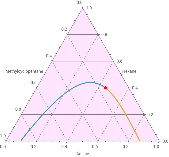
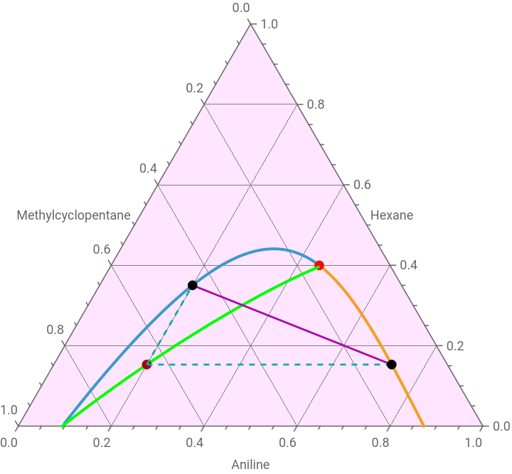
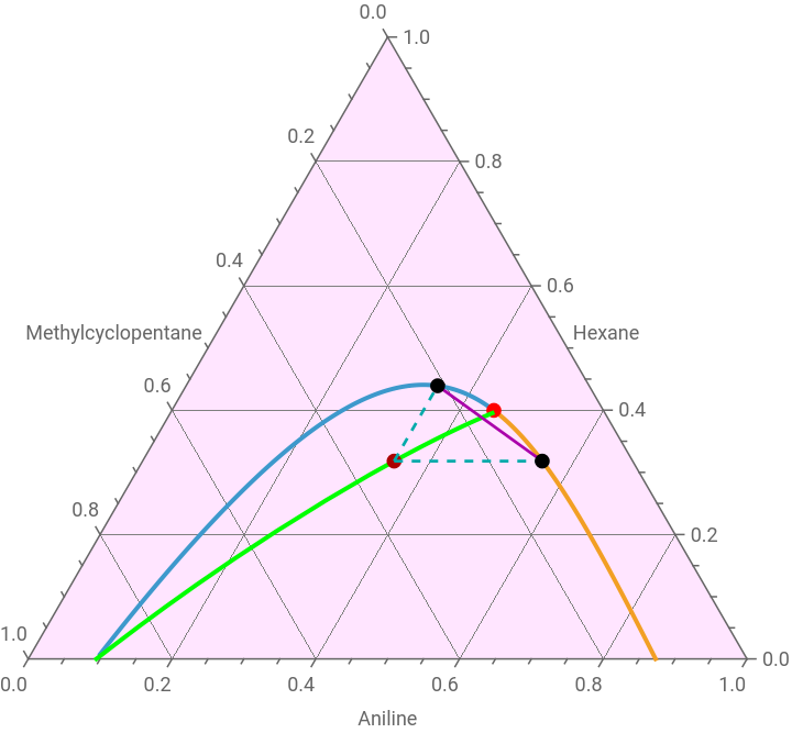
Consider the ternary system aniline-Tie Lines from a Conjugate Curve in Ternary LLE Diagram--hexane at (see Refs. 1-2). For temperatures above , this ternary system gives a type I liquid-liquid equilibrium (LLE) diagram. We use arc-length continuation to compute the LLE diagram (for details about this method see Refs. 3-4). In addition, the conjugate curve (shown in green) is superimposed on the same diagram. As we choose a point on the conjugate curve by setting the numerical value for x0 (i.e., 0.2, 0.35 or 0.15), the code constructs the corresponding tie line shown in magenta.
n
45
35°C
Gas constant in kcal/kmol*K
R=1.987;
Temperature in Kelvin
TK=273.15+45;
NRTL model
GAMMA1=Exp[(t21G21x2+t31G31x3)/(x1+G21x2+G31x3)+x1/(x1+G21x2+G31x3)(-(x2t21G21+x3t31G31)/(x1+G21x2+G31x3))+x2G12/(G12x1+x2+G32x3)(t12-(x1t12G12+x3t32G32)/(G12x1+x2+G32x3))+x3G13/(G13x1+G23x2+x3)(t13-(x1t13G13+x2t23G23)/(G13x1+G23x2+x3))]/.x31-x1-x2;GAMMA1p=Exp[(t21G21xp2+t31G31xp3)/(xp1+G21xp2+G31xp3)+xp1/(xp1+G21xp2+G31xp3)(-(xp2t21G21+xp3t31G31)/(xp1+G21xp2+G31xp3))+xp2G12/(G12xp1+xp2+G32xp3)(t12-(xp1t12G12+xp3t32G32)/(G12xp1+xp2+G32xp3))+xp3G13/(G13xp1+G23xp2+xp3)(t13-(xp1t13G13+xp2t23G23)/(G13xp1+G23xp2+xp3))]/.xp31-xp1-xp2;GAMMA2=Exp[(t12G12x1+t32G32x3)/(G12x1+x2+G32x3)+x1G21/(x1+G21x2+G31x3)(t21-(x2t21G21+x3t31G31)/(x1+G21x2+G31x3))+x2/(G12x1+x2+G32x3)(-(x1t12G12+x3t32G32)/(G12x1+x2+G32x3))+x3G23/(G13x1+G23x2+x3)(t23-(x1t13G13+x2t23G23)/(G13x1+G23x2+x3))]/.x31-x1-x2;GAMMA2p=Exp[(t12G12xp1+t32G32xp3)/(G12xp1+xp2+G32xp3)+xp1G21/(xp1+G21xp2+G31xp3)(t21-(xp2t21G21+xp3t31G31)/(xp1+G21xp2+G31xp3))+xp2/(G12xp1+xp2+G32xp3)(-(xp1t12G12+xp3t32G32)/(G12xp1+xp2+G32xp3))+xp3G23/(G13xp1+G23xp2+xp3)(t23-(xp1t13G13+xp2t23G23)/(G13xp1+G23xp2+xp3))]/.xp31-xp1-xp2;GAMMA3=Exp[(t13G13x1+t23G23x2)/(G13x1+G23x2+x3)+x1G31/(x1+G21x2+G31x3)(t31-(x2t21G21+x3t31G31)/(x1+G21x2+G31x3))+x2G32/(G12x1+x2+G32x3)(t32-(x1t12G12+x3t32G32)/(G12x1+x2+G32x3))+x3/(G13x1+G23x2+x3)(-(x1t13G13+x2t23G23)/(G13x1+G23x2+x3))]/.x31-x1-x2;GAMMA3p=Exp[(t13G13xp1+t23G23xp2)/(G13xp1+G23xp2+xp3)+xp1G31/(xp1+G21xp2+G31xp3)(t31-(xp2t21G21+xp3t31G31)/(xp1+G21xp2+G31xp3))+xp2G32/(G12xp1+xp2+G32xp3)(t32-(xp1t12G12+xp3t32G32)/(G12xp1+xp2+G32xp3))+xp3/(G13xp1+G23xp2+xp3)(-(xp1t13G13+xp2t23G23)/(G13xp1+G23xp2+xp3))]/.xp31-xp1-xp2;G12=Exp[-a12t12];G21=Exp[-a12t21];G13=Exp[-a13t13];G31=Exp[-a13t31];G32=Exp[-a32t32];G23=Exp[-a32t23];t13=A13+B13/TK;t23=A23+B23/TK;t12=A12+B12/TK;t32=A32+B32/TK;t31=A31+B31/TK;t21=A21+B21/TK;
NRTL parameters obtained from Aspen-Plus
param={a130.3,a120.20,a320.30,B12857.3718000,B212650.684300,B131410.932300,B312291.817900,B23190.1605000,B32-153.9573000,A12-1.969300000,A13-2.802700000,A230.0,A21-7.132100000,A31-5.248600000,A320.0};
In[]:=
X1i=0.5;X2i=0.1;sol=FindRoot[{GAMMA1x1GAMMA1pxp1,GAMMA2x2GAMMA2pxp2,GAMMA3(1-x1-x2)GAMMA3p(1-xp1-xp2),L+Lp1,x1L+xp1LpX1i,x2L+xp2LpX2i}/.param,{x2,0.193},{x1,0.058},{xp1,0.900},{xp2,0.035},{L,0.3},{Lp,0.8},AccuracyGoal10,MaxIterations5000];X1=0.5;
Arc-length continuation method
Eq1=GAMMA1x1GAMMA1pxp1/.x1x1[s]/.x2x2[s]/.xp1xp1[s]/.xp2xp2[s]/.LL[s]/.LpLp[s]/.X2X2[s]/.param;Eq2=GAMMA2x2GAMMA2pxp2/.x1x1[s]/.x2x2[s]/.xp1xp1[s]/.xp2xp2[s]/.LL[s]/.LpLp[s]/.X2X2[s]/.param;Eq3=GAMMA3(1-x1-x2)GAMMA3p(1-xp1-xp2)/.x1x1[s]/.x2x2[s]/.xp1xp1[s]/.xp2xp2[s]/.LL[s]/.LpLp[s]/.X2X2[s]/.param;Eq4=L+Lp1/.x1x1[s]/.x2x2[s]/.xp1xp1[s]/.xp2xp2[s]/.LL[s]/.LpLp[s]/.X2X2[s];Eq5=x1L+xp1LpX1/.x1x1[s]/.x2x2[s]/.xp1xp1[s]/.xp2xp2[s]/.LL[s]/.LpLp[s]/.X2X2[s];Eq6=x2L+xp2LpX2/.x1x1[s]/.x2x2[s]/.xp1xp1[s]/.xp2xp2[s]/.LL[s]/.LpLp[s]/.X2X2[s];Eq7=X2'[s]^2+x1'[s]^2+xp1'[s]^2+x2'[s]^2+xp2'[s]^2+L'[s]^2+Lp'[s]^21;
Auxiliary equation
sys={Eq1,Eq2,Eq3,Eq4,Eq5,Eq6,Eq7,X2[0]X2i,x1[0](x1/.sol),x2[0](x2/.sol),xp1[0](xp1/.sol),xp2[0](xp2/.sol),L[0](L/.sol),Lp[0](Lp/.sol),x1'[0]0,xp1'[0]0,x2'[0]0,xp2'[0]0,L'[0]0,Lp'[0]0,X2'[0]1};
Full DAE system of equations + initial conditions to be solved by NDSolve
In[]:=
SOL=Quiet@NDSolve[sys,{x1,x2,xp1,xp2,L,Lp,X2},{s,-10,10},AccuracyGoal5];lobound=a/.FindRoot[(x2[s]/.SOL/.sa)0,{a,0}];upbound=SOL[[1]][[1]][[2]][[1]][[1]][[2]];
DATA1=Table[{x1[s],x2[s],1-x1[s]-x2[s]}/.SOL,{s,lobound,upbound,0.01}];DATA2=Table[{xp1[s],xp2[s],1-xp1[s]-xp2[s]}/.SOL,{s,lobound,upbound,0.01}];Pt={{2,1},{0,Sqrt[3.]}}/2;
Type I liquid-liquid equilibrium (LLE) diagram - Plait point indicated in red
p0=Show[TernaryListPlot[{Flatten[DATA1,1],Flatten[DATA2,1]},Joined->True,PlotStyle->Thick,GridLines->Automatic,FrameLabel->{"Aniline","Hexane","Methylcyclopentane"},PlotRange->All,Method->{"Backdrop"->LightMagenta}],Graphics[{Red,PointSize[0.02],Point[Pt.{x1[s],x2[s]}/.SOL/.s->upbound]}]]
Out[]=
Plotting the conjugate curve shown in green
sconj1=ParametricPlot[Pt.{x1[s],xp2[s]}/.SOL,{s,upbound,lobound},PlotPoints100,PlotStyle{Green,Thick}];
Use the conjugate curve to get an interpolating function f in order to plot the dotted cyan lines in the various plots given below
sconj1b=ParametricPlot[{x1[s],xp2[s]}/.SOL,{s,upbound,lobound},PlotPoints100,PlotStyle{Green,Thick}];tbl=First[Cases[sconj1b,x_LineFirst@x,Infinity]];f=Interpolation[tbl];
In[]:=
x0=0.2;
In[]:=
srt=FindRoot[(x1[s]/.SOL)x0,{s,lobound}]
Out[]=
{s0.291489}
In[]:=
Show[p0,sconj1,Graphics[{PointSize[0.02],Darker@Red,Point[Pt.{x0,f[x0]}],Darker@Magenta,Thickness[0.004],Line[{Pt.{x1[s],x2[s]},Pt.{xp1[s],xp2[s]}}/.SOL/.srt],Dashed,Darker@Cyan,Line[{Pt.{x0,f[x0]},Pt.{x0,First[x2[s]/.SOL/.srt]}}],Line[{Pt.{x0,f[x0]},Pt.{First[xp1[s]/.SOL/.srt],f[x0]}}],Black,Point[Pt.{x0,First[x2[s]/.SOL/.srt]}],Point[Pt.{First[xp1[s]/.SOL/.srt],f[x0]}]}]]
Out[]=
In[]:=
x0=0.35;
In[]:=
srt=FindRoot[(x1[s]/.SOL)x0,{s,lobound}]
Out[]=
{s0.700312}
In[]:=
Show[p0,sconj1,Graphics[{PointSize[0.02],Darker@Red,Point[Pt.{x0,f[x0]}],Darker@Magenta,Thickness[0.004],Line[{Pt.{x1[s],x2[s]},Pt.{xp1[s],xp2[s]}}/.SOL/.srt],Dashed,Darker@Cyan,Line[{Pt.{x0,f[x0]},Pt.{x0,First[x2[s]/.SOL/.srt]}}],Line[{Pt.{x0,f[x0]},Pt.{First[xp1[s]/.SOL/.srt],f[x0]}}],Black,Point[Pt.{x0,First[x2[s]/.SOL/.srt]}],Point[Pt.{First[xp1[s]/.SOL/.srt],f[x0]}]}]]
Out[]=
References
References
[2] J. D. Seader, E. J. Henley, and D. K. Roper, Separation Process Principles: Chemical and Biochemical Operations, 3rd ed., New York: Wiley, 2011.
[3] H. Binous and A. Bellagi, Calculation of Ternary Liquid - Liquid Equilibrium Data using Arc - Length Continuation, Engineering Reports, 3 (2), 2021.
[4] H. Binous , K. Mejbri , and A. Bellagi , Application of graduate-level numerical tools to teach phase equilibria of liquid ternary systems. Comput Appl Eng Educ. 2021; 29: 1589–1601. https://doi.org/10.1002/cae.22411
CITE THIS NOTEBOOK
CITE THIS NOTEBOOK
Tie lines from a conjugate curve in ternary LLE diagram
by Housam Binous
Wolfram Community, STAFF PICKS, April 10, 2026
https://community.wolfram.com/groups/-/m/t/3681925
by Housam Binous
Wolfram Community, STAFF PICKS, April 10, 2026
https://community.wolfram.com/groups/-/m/t/3681925