Introduction
Introduction
Gases, liquids, and solids can be modeled as large collections of hard spheres that scatter elastically with one another when they come into contact. Hard sphere models, though ostensibly quite simple, contain valuable insights and surprising nuance. In this project, we construct a hard sphere model simulation. From this simulation, we derive two types of networks from the collisions between particles. We then explore these networks.
In particular, we are interested here in the types of networks that arise from the connections made by collisions in these models. We call the first type of graph we consider a “scattering graph.” The nodes in the scattering graph represent individual particles, and the edges connecting them represent collisions between those particles. The network below is the scattering graph for the simulation you see above.
In[]:=
GraphcollisionsToScatteringGraph[collsBigBox],
Out[]=
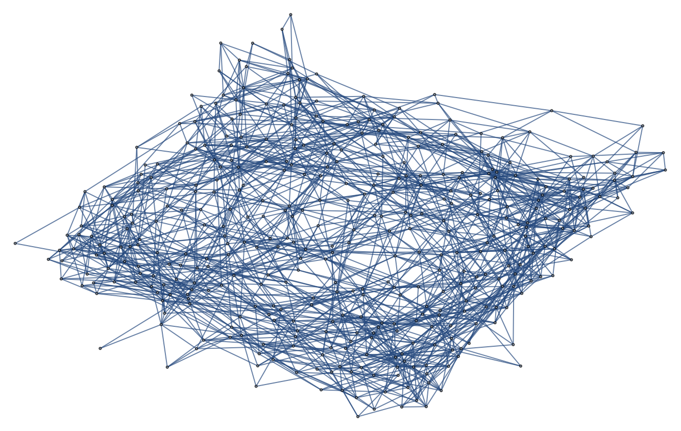
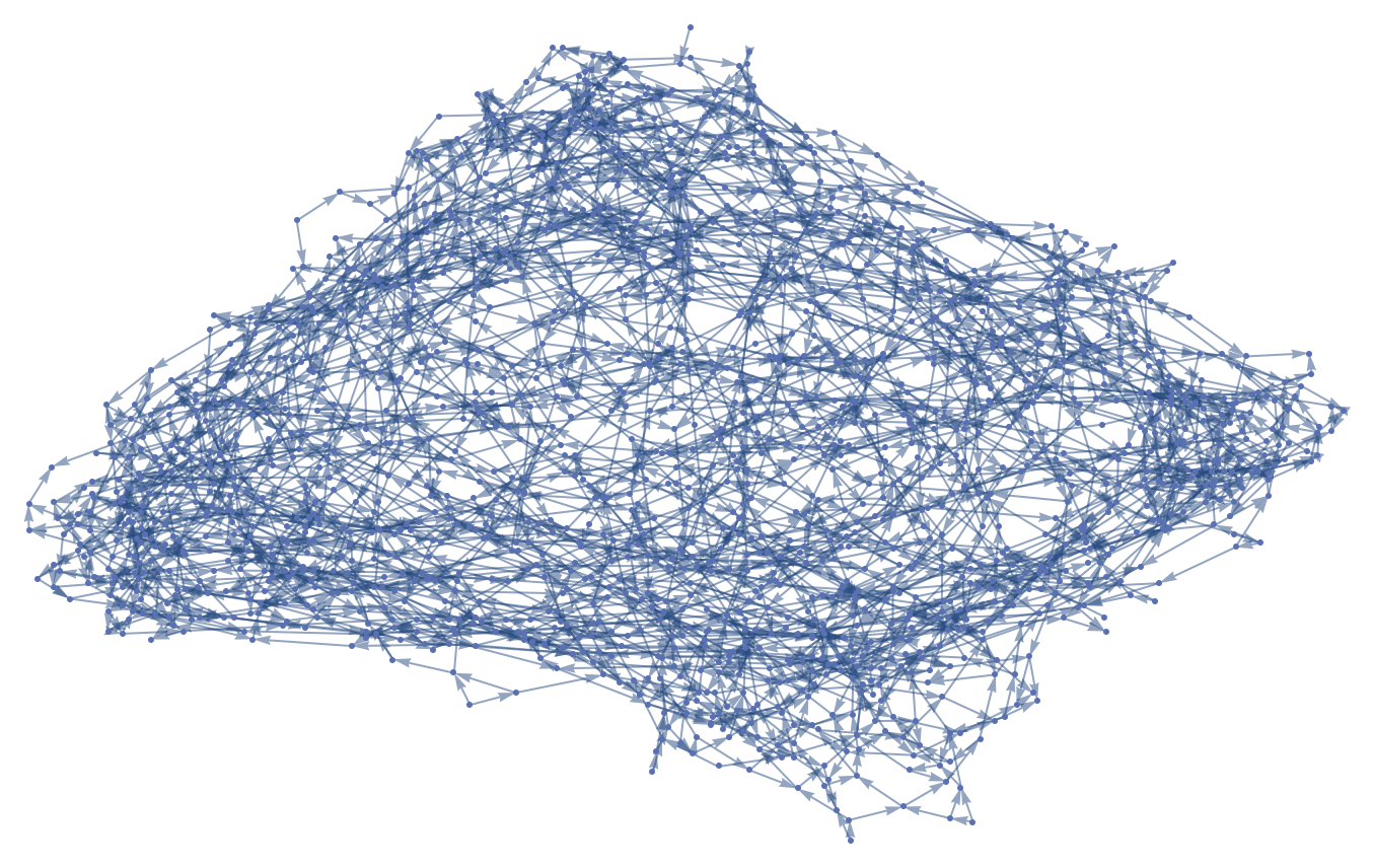
The other type of graph we derive from these simulations are “causal graphs.” The causal graph derived from this simulation is shown below. In these directed graphs, nodes represent collisions, and directed edges indicate that a particle participated in the original collision, and then in the destination collision. represent temporal ordering of collisions.
In[]:=
GraphcollisionsToCausalGraph[collsBigBox],
Out[]=
Scattering Graphs
Scattering Graphs
We are not aware of the properties of the scattering graphs derived from hard sphere models. For larger simulations (e.g. below, with 1000 particles), the networks appear to exhibit at least some non-trivial structure. We attempt to investigate this structure by estimating the effective dimension of a scattering graph.
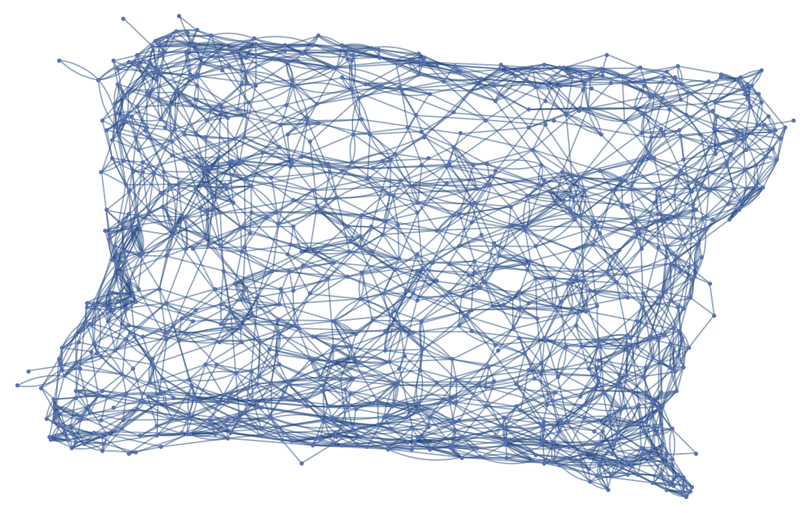
Using our compiled simulation, we generated the animation at the top of this notebook. We construct the associated scattering graph from the list of collisions in that simulation, collsBigBox, which takes the form .
{{,,time},...}
particle
1
particle
2
In[]:=
GraphDeleteDuplicates[#〚1〛#〚2〛]&/@collsBigBox,
Out[]=
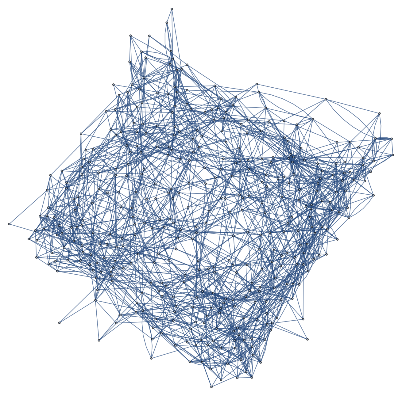
Having constructed the graph, we can attempt to derive its dimension by measuring how the number of nodes scales with graph distance (on average).
In[]:=
scatteringGraphScaling[graph_,verToSample_:100]:=Mean/@Table[Length[VertexOutComponent[graph,#,n]]&/@RandomSample[VertexList[graph],UpTo[verToSample]],{n,GraphDiameter[graph]}]
Applying this function to the collisions from above
In[]:=
scaling=scatteringGraphScaling[collisionsToScatteringGraph[collsBigBox]];
In[]:=
ListLogLogPlot[{Range@Length@scaling,scaling},FrameTrue,FrameLabel(Style[#,Black,12]&/@{"Graph Distance","# Nodes"}),PlotLabelStyle["Scattering Graph Scaling Relationship",Black,14]]
Out[]=
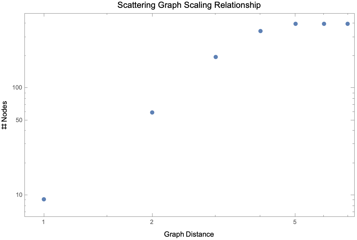
Clearly, our technique for measuring dimension fails near the boundary of our graph (indicated by the horizontal asymptote above); however, in the (ostensibly) linear regime we can estimate the effective dimension of the scattering graph.
In[]:=
fit=FindFit[Log[Transpose[{Range[Length[scaling]],scaling}]][[;;4]],mx+b,{m,b},x]
Out[]=
{m2.65207,b2.24931}
In[]:=
Show[ListLogLogPlot[scaling,FrameTrue,FrameLabel(Style[#,Black,12]&/@{"Graph Distance","# Nodes"}),PlotLabelStyle["Scattering Graph Scaling Relationship",Black,14]],Plot[mx+b/.fit,{x,0,5},PlotStyleDirective[Black,Dashed]]]
Given that the slope of this line is our estimate for the graph’s effective dimension, our analysis indicates that the graph has an effective dimension between two and three.
(We note that this analysis could probably be made more robust by using larger graphs. These computations are too expensive at present, but are not overwhelmingly expensive.)
(We note that this analysis could probably be made more robust by using larger graphs. These computations are too expensive at present, but are not overwhelmingly expensive.)
Causal Graphs
Causal Graphs
In addition, we are not aware of the properties of causal graphs derived from hard sphere models. For simulations involving large numbers of particles (e.g. below, with 1000 particles), the causal graphs appear to take on manifold-like structure. This type of structure is being explored extensively in the Wolfram Physics Project in the context of fundamental physics. Similarly to the scattering graphs, we investigate the dimension of the causal graph derived from the simulation above. In this case, however, we are interested in the dimensions of light cones in the casual graph.
(Conceptually, it is helpful to arrange the causal graph using “LayeredDigraphEmbedding” because, roughly speaking, time proceeds down the screen.)
We then construct a function to highlight lightcones in our graph. We define lightcones to be the VertexOutComponent[] of a particular vertex, out to a certain depth.
We depict a few light cones below, highlighted in red.
In some hard sphere systems (e.g. below, a small box with high density), light cones can propagate quickly to encompass the entire future of the system.
However, in the previous images, we see that in some systems light cones may extend for long durations without encompassing the whole system.
When one considers these networks in the context of the Wolfram Physics Project, one is often interested in the effective dimension of the causal graph. Just as with the scattering graph, we estimate the dimension by measuring how the number of nodes scales. This time, however, we measure how the number scales in time.
Unlike in the scattering graph case, there appears to be no trend whatsoever here. We confirm this with a log-log plot.
Thus, it appears the the causal graphs derived from our simulation do not have a well-defined dimension. This was not obvious from simply observing them!
Arc-Length Distributions
Arc-Length Distributions
This particular path of exploring effective dimension is not the only interesting question that can be asked about these networks. We also used the causal graph to answer the following question, “How far, on average, do particles move before scattering, at a given density?”
Each edge in the causal graph indicates that a particle has undergone two collisions in sequence, without undergoing any collision in between. Thus, by extracting the particle’s speed and the duration associated with the edge, we can determine the (arc-length) distance that that particle travels between collisions.
By applying this analysis to an entire causal graph, we can investigate the distribution of how far particles move, at a given density.
Below, we show the scaling relationship measured for a variety of box sizes.
Below, we show the scaling relationship measured for a variety of box sizes.
Evidently, the mean distance traveled decays exponentially with density.
Rather than simply looking at the mean distance travelled, we can look at the whole distribution. Below, we display the PDFs for the data for box radius 20:
We remark that, although the axes vary considerably in the images above, most of the distributions decay monotonically below a certain density. It is interesting to note that this pattern may change above density = 0.65.
To investigate these distributions more precisely, we plot the logs of the PDFs.
To investigate these distributions more precisely, we plot the logs of the PDFs.
Higher Dimensions
Higher Dimensions
Another potentially fruitful line of inquiry would be to explore higher dimensions. We designed our code to run in any dimension, not just two. It is not at all easy to predict how the networks will behave in higher dimensions.
We can visualize a simulation in 3-dimensions.
We can visualize a simulation in 3-dimensions.
But it is hard to imagine what is taking place in this five dimensional box:
It would be interesting to see how our analysis differs for higher dimensions. This suggests another line for future inquiry.
Concluding Remarks
Concluding Remarks
The networks derived from hard sphere simulations appear to exhibit non-trivial structure. In this notebook, we briefly explored some aspects of these networks, focusing particularly on their spatial dimension. However, it seems highly likely that there are many new things to learn from these networks.