I have added some examples of how the Chebyshev approximation algorithms work in arbitrary precision. These demonstrate some of the pure mathematics at work in the Chebyshev polynomial approximations.
Reconstruction of a Random Polynomial
Reconstruction of a Random Polynomial
In[]:=
Clear[randomPoly];randomPoly::usage="randomPoly[n] generates a polynomial Function[] with n terms having rational coefficients";randomPoly[n_]:=Module[{rr},rr=#1/#2&@@@RandomInteger[{-100,100},{n,2}];Evaluate[Sum[rr[[i+1]]#^i,{i,0,n-1}]]&];
In[]:=
fn=randomPoly[20];fn[x]
Out[]=
------+69+--+++++--++-
32
41
14x
43
67
2
x
78
3
3
x
22
97
4
x
47
97
5
x
35
6
x
11
7
x
91
5
8
x
3
5
9
x
12
37
10
x
20
15
11
x
61
33
12
x
20
39
13
x
79
22
14
x
97
8
15
x
97
20
16
x
7
96
17
x
49
31
18
x
97
16
19
x
19
Here is the plot of a random polynomial over the range {-1, 1}. By the plot the interval may not seem to carry enough information, but the interval carries all the information needed to recover the polynomial with a Chebyshev approximation. Each Chebyshev polynomial used in the approximation has all its roots in the interval {-1, 1} and they are real, so each polynomial fragment can be solved. This is a good demonstration of the power of Mathematica’s symbolic representation. The algorithms use Cos[] functions but the polynomial coefficients all come out rational numbers. The Chebyshev polynomials all have integer coefficients.
In[]:=
Plot[fn[x],{x,-1,1},PlotRange->All]
Out[]=
Here are the Chebyshev coefficients for the function on the interval, {-1, 1}. Note that 22 terms were sought but the last two were zero, and all subsequent coefficients should be zero.
In[]:=
cc=ChebyCoeff[fn,{-1,1},22]//FullSimplify
Out[]=
,-,,-,,,,,-,,-,,-,,-,-,-,-,,-,0,0
108665407450493
2786857615360
1827119206840085
1153769827065856
43085087841
1401487360
12059707081967
26831856443392
704862613
56020992
43648487901
435582085120
19872389
9535488
21932002655
174232834048
1226189
23838720
1685522665
40207577088
406313
15892480
214741281
23454419968
101239
13905920
6139143
6151979008
88495
88997888
3593
77873152
1927
44498944
25
802816
31
12713984
1
311296
The polynomial is reconstructed using ChebyFn and non-zero terms; it is identical to original function which has domain, {-∞, ∞}.
In[]:=
fn1=ChebyFn[cc,{-1,1},20]//ExpandAll//FullSimplify;fn1[x]FullSimplify[fn1[x]==fn[x]]
Out[]=
------+69+--+++++--++-
32
41
14x
43
67
2
x
78
3
3
x
22
97
4
x
47
97
5
x
35
6
x
11
7
x
91
5
8
x
3
5
9
x
12
37
10
x
20
15
11
x
61
33
12
x
20
39
13
x
79
22
14
x
97
8
15
x
97
20
16
x
7
96
17
x
49
31
18
x
97
16
19
x
19
Out[]=
True
If you try to reconstruct the polynomial with fewer terms than the original, you will not get an exact representation, but note that the lower order coefficients are the same and exact. The higher order coefficients are different from the exact polynomial.
In[]:=
cc1=ChebyCoeff[fn,{-1,1},15]//FullSimplify
Out[]=
,-,,-,,,,,-,,-,,-,,-
108665407450493
2786857615360
1827119206840085
1153769827065856
43085087841
1401487360
12059707081967
26831856443392
704862613
56020992
43648487901
435582085120
19872389
9535488
21932002655
174232834048
1226189
23838720
1685522665
40207577088
406313
15892480
65304254131
7130143670272
3240733
444989440
3165359
3075989504
84641
88997888
In[]:=
Take[cc,15]-cc1
Out[]=
0,0,0,0,0,0,0,0,0,0,0,-,,-,-
1
311296
31
12713984
25
802816
1927
44498944
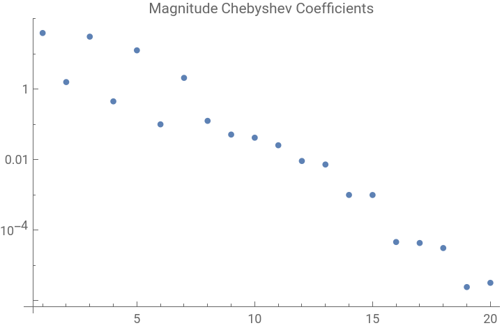
The Chebyshev coefficients generally decrease in magnitude for higher orders of the polynomial. If the polynomial is on the domain {-1, 1}, these magnitudes show roughly the error at the level of the last term. When constructing a polynomial for use in approximation you will get a better estimate of the lower order coefficients if you take n greater than the polynomial order you need then truncate the list to the number of terms required.
In[]:=
ListLogPlot[Abs[cc],PlotRange->All,PlotLabel->"Magnitude Chebyshev Coefficients"]
Out[]=
Exponential Function
Exponential Function
For the exponential function the Chebyshev approximation finds the Taylor series with the coefficients asymptotically approaching the values 1/k! Other trigonometric series also approach the Taylor series.
Below are coefficients for 5, 10, 20 terms of an approximation to the exponential function. As n increases so does the number of terms used to construct each coefficient. The first coefficient of each series is shown.
In[]:=
c51=ChebyCoeff[Exp[#]&,{-1,1},5];c101=ChebyCoeff[Exp[#]&,{-1,1},10];c201=ChebyCoeff[Exp[#]&,{-1,1},20];c51[[1]]c101[[1]]c201[[1]]
Out[]=
2
5
--
5
8
5
8
5
8
5
8
-+
5
8
5
8
5
8
5
8
Out[]=
1
5
-
1
2
1
2
-Cos
π
20
Cos
π
20
-Cos
3π
20
Cos
3π
20
-Sin
π
20
Sin
π
20
-Sin
3π
20
Sin
3π
20
Out[]=
1
10
-Cos
π
40
Cos
π
40
-Cos
3π
40
Cos
3π
40
-Cos
π
8
Cos
π
8
-Cos
7π
40
Cos
7π
40
-Cos
9π
40
Cos
9π
40
-Sin
π
40
Sin
π
40
-Sin
3π
40
Sin
3π
40
-Sin
π
8
Sin
π
8
-Sin
7π
40
Sin
7π
40
-Sin
9π
40
Sin
9π
40
The terms appear to be approaching a limit as n increases.
In[]:=
N[{c51[[1]],c101[[1]],c201[[1]]},50]//TableForm
Out[]//TableForm=
2.5321317544028374552617413870695453224222433437902 |
2.5321317555040166711964876636950407476073183298786 |
2.5321317555040166711964892504294350752153406227099 |
The function is progressively increasing toward a limit.
In[]:=
dff=Differences[N[ChebyCoeff[Exp[#]&,{-1,1},#][[1]]&/@Table[2^i,{i,4,10}],1500]];#2<#1&@@@Partition[%,2,1]N[Log[10,dff]]dff[[-1]]
Out[]=
{True,True,True,True,True}
Out[]=
{-44.4478,-107.766,-253.515,-583.395,-1320.07,Indeterminate}
Out[]=
0.×
-1500
10
In fact when the terms are converted to the polynomial they represent , it is apparent that they are approaching the Taylor series coefficients of the exponential function.
In[]:=
ts=CoefficientList[Series[Exp[x],{x,0,19}]//Normal,x]N[CoefficientList[ChebyFn[c51,{-1,1},5][x],x],30]N[CoefficientList[ChebyFn[c101,{-1,1},10][x],x],30]N[CoefficientList[ChebyFn[c201,{-1,1},20][x],x],30]ListLogPlot[Abs[%-ts],GridLines->Automatic,PlotRange->All,PlotLabel->"Magnitude Difference from Taylor Series Coefficient"]
Out[]=
1,1,,,,,,,,,,,,,,,,,,
1
2
1
6
1
24
1
120
1
720
1
5040
1
40320
1
362880
1
3628800
1
39916800
1
479001600
1
6227020800
1
87178291200
1
1307674368000
1
20922789888000
1
355687428096000
1
6402373705728000
1
121645100408832000
Out[]=
{1.00000000000000000000000000000,0.997317242686734291612227629278,0.499556175688009363906997129143,0.177334605648645961488002729322,0.0434341049531041218063256772353}
Out[]=
{1.00000000054851414806409239382,1.00000000004972013002250746233,0.499999972578426478799207261773,0.166666664180977575103662956196,0.0416668858656544305289075545256,0.00833335320551637159776973835375,0.00138827620546403191973299915044,0.000198357138755534687437527825951,0.0000254990645139262584353351601723,2.81901879279295859224136724583×}
-6
10
Out[]=
{0.999999999999999999999999207490,0.999999999999999999999999962297,0.500000000000000000000158500258,0.166666666666666666666674207211,0.0416666666666666666614364441246,0.00833333333333333333308450779910,0.00138888888888888895582882004410,0.000198412698412698415883078996557,0.0000248015873015868665489328887017,2.75573192239856836801755844743×,2.75573192241482649725903398971×,2.50521083855189710830172004696×,2.08767569509785673732708785116×,1.60590438192702344425842232013×,1.14707507835503670320148046655×,7.64716619926595627180444030302×,4.77903698079475584714306001093×,2.81124771399455356522512022840×,1.58260068143905535400914107032×,8.31905802133232954791863936581×}
-6
10
-7
10
-8
10
-9
10
-10
10
-11
10
-13
10
-14
10
-15
10
-16
10
-18
10
The lowest order coefficients have the greatest accuracy. The accuracy can be further improved by increasing n, but clearly there are diminishing returns.
The errors using ChebyEval[].
The error of the approximation at precision, 30, is about the same as the Taylor series of the same order.
If the precision of the coefficients is not preset, errors accumulate from multiplying the large number of terms in each polynomial coefficient using $MachinePrecision.
Complex functions of a real variable also work.
Complex functions of a real variable also work.
Here is the complex function for a unit circle centered at 0+0 . This is basically the same as the exponential demonstration above.
Here is the plot the approximation to a circle with only order 9 polynomial is quite good.
The ChebyEval function can also handle complex coefficients.
The error as distance from the origin.
The unit circle as a Taylor series on the real plane doesn’t work well at all.