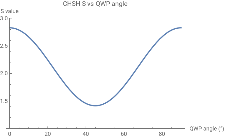
In their seminal 1995 paper, Kwiat et al . demonstrated how a maximally entangled photon pair could be generated using Type - II SPDC and tuned it into any of the four Bell states by introducing a relative phase between the and components . Remarkably, they noted “Somewhat surprisingly, a net phase shift of may be obtained by a 90 ° rotation of a quarter-wave plate in one of the paths," allowing precise control over the entanglement phase using birefringent optics . This notebook simulates the CHSH - parameter as a function of QWP angle using the Jones matrix formalism, and finds at 0 ° and 90°, and a minimum of at 45 ° .
|HV〉
|VH〉
π
S
S2.828
S1.414
Method
Method
To simulate the experimental tuning of Bell states via a quarter-wave plate (QWP), we implemented a Mathematica function that computes the CHSH -parameter as a function of the QWP rotation angle (in radians).The QWP is modeled using the standard Jones matrix:where is the rotation matrix acting on the polarization basis. This transformation is applied to one arm of the entangled Bell state: and the complex phases are removed by taking the element-wise absolute value of the resulting amplitudes.We evaluate the CHSH -parameter by computing the correlation expectation values using the standard four-setting scheme: with measurement angles (in radians): 0, , , -.The function returns the value of for a given QWP angle . We generate the CHSH curve by evaluating over the interval The resulting -curve is symmetric, with predicted values such as , and . While only the extremal points at and were explicitly noted in the experimental observations of Kwiat et al. (1995), this simulation illustrates the full continuous dependence of the CHSH parameter on the QWP rotation angle. These values correspond to maximal violation at linear polarization and minimal violation at circular projection mismatch in one of the arms.
S[QWPtheta_]
S
θ
Q(θ)R(-θ)
R(θ),
1 | 0 |
0 | i |
R(θ)
(Q(θ)|〉⊗ |〉 + Q(θ)|〉 ⊗|〉 ),
ψ
QWP
1
2
H
1
V
2
V
1
H
2
S
E(,)
θ
1
θ
2
SE(,)-E+E,+E,,
θ
1
θ
2
†
θ
1
θ
2
θ
1
†
θ
2
†
θ
1
†
θ
2
θ
1
†
θ
1
π
4
θ
2
π
8
†
θ
2
π
8
S[QWPtheta]
S
θ
S
[,]
◦
0
◦
90
S
S()S()2.828
◦
0
◦
90
S()1.414
◦
45
◦
0
◦
90
S
Reference
Reference
Kwiat, P.G., Mattle, K., Weinfurter, H., Zeilinger, A., Sergienko, A.V. and Shih, Y. (1995) “New High-Intensity Source of Polarization-Entangled Photon Pairs,” Physical Review Letters, 75, pp. 4337–4341.
Input Block
Input Block
In[]:=
ClearAll["Global`*"](*Definepolarizationbasisvectors*)H={1,0};V={0,1};(*Definelinearpolarizerstateatangleθ*)Polarizer[theta_]:=Cos[theta]H+Sin[theta]V;(*DefineJonesMatrixforQWPoperatoratarbitraryangleθinradians*)QWP[theta_]:=Module[{R,Rinv},R={{Cos[theta],-Sin[theta]},{Sin[theta],Cos[theta]}};Rinv=Transpose[R];(*return*)Rinv.{{1,0},{0,I}}.R](*DefineCoincidenceprobability*)CoinProb[theta1_,theta2_]:=Module[{pol1=N[Polarizer[theta1]],pol2=N[Polarizer[theta2]],proj},proj=Flatten[KroneckerProduct[pol1,pol2]];(*return*)N[Conjugate[proj].psiBellQWP]^2](*DefineOrthogonalangle:90°rotation*)Perp[theta_]:=Mod[theta+Pi/2,Pi](*DefineExpectationvalueE(θ1,θ2)*)ExpVal[theta1_,theta2_]:=Module[{a=N[CoinProb[theta1,theta2]],b=N[CoinProb[Perp[theta1],Perp[theta2]]],c=N[CoinProb[theta1,Perp[theta2]]],d=N[CoinProb[Perp[theta1],theta2]]},(*return*)(a+b-c-d)/(a+b+c+d)]S[QWPtheta_]:=Module[{Q,Hqwp,Vqwp,e1,e2,e3,e4},Q=QWP[QWPtheta];(*ApplyQWPtoarmAonly*)Hqwp=Q.H;Vqwp=Q.V;(*CreatetheentangledstateafterQWPinarmA*)(*psiBellQWPisglobalsothatCoinProb[theta1_,theta2_]canuseit*)psiBellQWP=Abs[1/Sqrt[2](Flatten[KroneckerProduct[Hqwp,V]]+Flatten[KroneckerProduct[Vqwp,H]])];(*Computeexpectationvalues*)e1=ExpVal[t1,t2];e2=ExpVal[t1p,t2];e3=ExpVal[t1,t2p];e4=se4*ExpVal[t1p,t2p];(*ComputeCHSHSvalueandreturnit*)Abs[e1-e2+e3+e4]](*CHSHanglesinradians*)t1=0;t1p=Pi/4;t2=Pi/8;t2p=-Pi/8;se4=1;Print" 0, , , -. "Print["S[0]=",S[0]," S[Pi/8]=",S[Pi/8]," S[Pi/4]=",S[Pi/4]]Plot[S[θDegree],{θ,0,90},AxesLabel->{"QWP angle (°)","S value"},PlotRange->{1,3},PlotLabel->"CHSH S vs QWP angle",PlotStyle->Thick](*LocalHiddenVariableSimmulation*)ClearAll["Global`*"](*Numberoftrials*)nSamples=10;(*Hiddenvariablemodel:randomλin[0,2π]*)lambdas=RandomReal[{0,2Pi},nSamples];(*Localdeterministicresponsefunction:±1*)A[theta_,lambda_]:=Sign[Cos[theta-lambda]];B[theta_,lambda_]:=Sign[Cos[theta-lambda]];(*ExpectationvaluefromLHVmodel*)ExpValLHV[theta1_,theta2_]:=Mean[A[theta1,#]*B[theta2,#]&/@lambdas](*ComputeCHSHSfromclassicalLHV*)S:=Module[{t1,t1p,t2,t2p,e1,e2,e3,e4},t1=Pi/4;t1p=3Pi/4;t2=Pi/8;t2p=3Pi/8;e1=ExpValLHV[t1,t2];e2=ExpValLHV[t1p,t2];e3=ExpValLHV[t1,t2p];e4=ExpValLHV[t1p,t2p];e1-e2+e3+e4]Print[" "]Print[" "]Print["CHSH S (LHV simulation) = ",N[S,4]]
θ
1
†
θ
1
π
4
θ
2
π
8
†
θ
2
π
8
θ
1
†
θ
1
π
4
θ
2
π
8
†
θ
2
π
8
S[0]=2.82843 S[Pi/8]=2.12132 S[Pi/4]=1.41421
Out[]=