We analyse the flavour profiles of 86 Scotch single malt distilleries — each scored 0–4 on 12 flavour dimensions by expert tasters — using hierarchical clustering to build a phylogenetic tree of whisky. The cophenetic distance from this tree is automatically an ultrametric (satisfying the strong triangle inequality d(x,z) ≤ max(d(x,y), d(y,z))), and we show that this ultrametric can be encoded as a p-adic distance on a base-3 number tree, connecting a 200-year-old piece of algebraic number theory (Hensel 1897) to a 21st-century tasting panel.
The analysis reveals that the ultrametric tree is shaped primarily by the Medicinal and Smoky dimensions (permutation importance 0.51 and 0.44), is significantly predicted by geography (Mantel r = 0.17, p = 0.004), and is more of a “cask tree” than a “terroir tree” (cluster purity 0.72 vs 0.60). UPGMA linkage produces the best-fitting ultrametric (cophenetic correlation 0.80), and 8 of 12 principal components suffice to capture 90% of flavour variance.
Audience: the notebook is written for two overlapping audiences. Each section opens with an intuitive explanation requiring no background, then deepens into the mathematics (metric spaces, p-adic valuations, Moran’s I, ANOVA). Whisky enthusiasts will recognise the distillery names; mathematicians will recognise the topology.
1. What makes Scotch whisky different?
1. What makes Scotch whisky different?
Scotch single malt whisky is a fermented, distilled, and barrel-aged spirit produced at a single distillery in Scotland from malted barley, water, and yeast. Its flavour depends on a chain of production decisions: the barley variety, whether the malt is dried over peat smoke, the shape of the copper pot stills, the duration and temperature of fermentation, the type of oak cask used for ageing, the climate of the warehouse, and the number of years the spirit spends in wood.
Despite this complexity, expert tasters consistently report that Scotch single malts cluster into recognisable flavour families that partially align with geography: the heavily peated malts of Islay, the light and floral Lowland whiskies, the honey-sweet Speyside core, and the diverse Highland fringe. The question this notebook asks is: what is the right mathematical structure for these flavour families? Are they flat clusters (like k-means)? Or do they form a nested hierarchy (like a phylogenetic tree)?
We will show that the answer is unambiguously hierarchical, and that the natural distance on the resulting tree is an ultrametric — a metric so strong that every triangle is isoceles. This is the same structure that underlies the p-adic numbers, the Tree of Life in biology, and the nested ball topology of non-Archimedean analysis. Whisky, it turns out, lives in p-adic space.
2. The data: 86 distilleries, 12 flavour dimensions
2. The data: 86 distilleries, 12 flavour dimensions
The dataset comes from David Wishart’s classification of 86 Scotch single malt distilleries, published through the University of Strathclyde’s Nessie outreach project. Each distillery is scored 0–4 on 12 flavour dimensions by expert tasters: Body, Sweetness, Smoky, Medicinal, Tobacco, Honey, Spicy, Winey, Nutty, Malty, Fruity, Floral.
Reproducible setup. Every figure below is generated by a single function call into the companion package whisky_figures.wl (in the same folder as this notebook). Evaluate the cell below once to import the package and prepare the shared objects: the flavour data, the complete-linkage merges tree, and the per-distillery caskTypes. Every later cell is exactly the call that produces its figure.
A note on the data. The flavour dataset is not redistributed with this notebook. LoadData[] downloads it on first use from its original public home — David Wishart’s classification, hosted by the University of Strathclyde’s Nessie outreach project (see §12) — and caches it locally, so the first evaluation needs an internet connection. The cached figures below already render without any data or evaluation.
In[]:=
SetDirectory[NotebookDirectory[]];Get["whisky_figures.wl"];(*LoadData[]downloadsthedatasetfromtheStrathclyde"Nessie"*)(*outreachpageonfirstuseandcachesitlocally(seeSection12).*)data=LoadData[];(*86×12flavourscores+geo+region*)merges=BuildMerges[data["flavours"]];(*complete-linkagetree*)caskTypes=LoadCaskTypes[data["names"]];(*primarycaskperdistillery*)n=Length[data["names"]];
The 86 distilleries span six official Scotch whisky regions: Speyside (42 distilleries), Highland (20), Islay (7), Islands (5), Lowland (3), and Campbeltown (2). The data also includes geographic coordinates (British National Grid), which we use in §8 for the spatial autocorrelation analysis.
In[]:=
RadarByRegion[data]
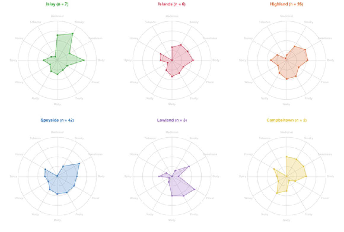
Figure 2.1 Mean flavour profiles by Scotch whisky region (radar charts). Islay (green) is dominated by Smoky, Medicinal, and Body; Speyside (blue) by Sweetness, Honey, and Fruity; Lowland (purple) by Floral and Fruity. These profiles hint at the hierarchical structure we are about to formalise.
The chemistry behind the scores. Each of the 12 flavour dimensions corresponds to families of volatile organic compounds produced during malting, fermentation, distillation, and maturation. Smoky and Medicinal arise from phenolic compounds (phenol, guaiacol, cresol) introduced when barley is kilned over peat. Sweet is driven by vanillin (from oak casks) and maltol. Fruity comes from esters (isoamyl acetate, ethyl hexanoate). The molecular structures below give a tangible chemical grounding for the 12-dimensional flavour space we are about to explore.
In[]:=
MoleculeGrid[]
Out[]=
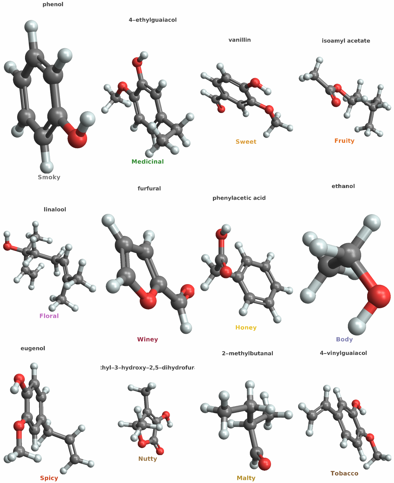
Figure 2.2 The chemistry of Scotch whisky: one key molecule per flavour dimension, rendered with MoleculePlot3D. From phenol (Smoky) to 4-vinylguaiacol (Tobacco), these compounds are the molecular basis of the flavour scores.
In[]:=
FlavourHeatmap[data,merges]
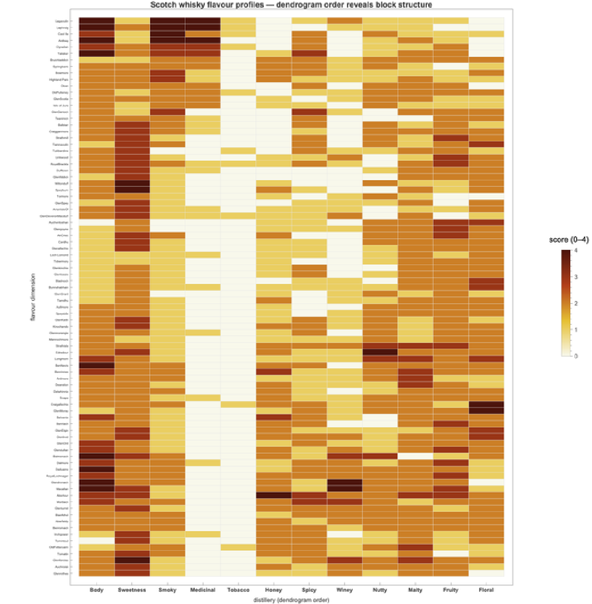
Figure 2.3 The 86 × 12 flavour matrix, sorted by dendrogram order (the ultrametric tree we build in §4). The block-diagonal structure is immediately visible: clusters of distilleries share similar flavour profiles, and the dendrogram order reveals these blocks.
3. What is an ultrametric?
3. What is an ultrametric?
The standard triangle inequality. A metric (distance function) d on a set X must satisfy four axioms: non-negativity, identity of indiscernibles, symmetry, and the triangle inequality:
d(x,z)≤d(x,y)+d(y,z)
This says: the direct path from x to z is never longer than a detour through y. Euclidean distance satisfies this. So does Manhattan distance, Hamming distance, and essentially every distance measure used in machine learning.
The ultrametric strengthening. An ultrametric replaces the sum with a maximum:
d(x,z)≤max(d(x,y),d(y,z))
This is strictly stronger: it implies the ordinary triangle inequality (since max ≤ sum) but says much more. The geometric consequence is startling: every triangle is isoceles, with the two longer sides equal. Proof: suppose d(x,y) > d(y,z). Then d(x,z) ≤ max(d(x,y), d(y,z)) = d(x,y), and d(x,y) ≤ max(d(x,z), d(z,y)) = d(x,z) (since d(x,z) ≥ d(z,y) would force d(x,y) ≤ d(x,z) ≤ d(x,y)), giving d(x,y) = d(x,z). The triangle {x, y, z} has two equal sides — and the third is the shortest.
UltrametricTriangle[data,merges]
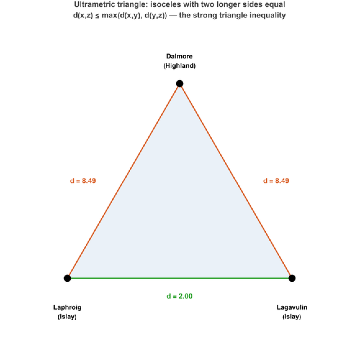
Figure 3.1 The ultrametric triangle in action: Laphroig and Lagavulin (both Islay peated malts) are close (cophenetic distance 2.00), while both sit at exactly the same distance from Dalmore (8.49). The triangle is isoceles with the two longer sides equal — the hallmark of an ultrametric.
Why ultrametric = tree-like. In an ultrametric space, every ball B(x, r) = {y : d(x,y) ≤ r} has the property that every point is a centre: if y ∈ B(x, r), then B(y, r) = B(x, r). Two balls are either disjoint or one contains the other. This means the family of all balls forms a rooted tree under inclusion — and the ultrametric distance between two points equals the radius of the smallest ball containing both. An ultrametric space IS a tree.
4. Building the tree: hierarchical clustering
4. Building the tree: hierarchical clustering
We compute the pairwise Euclidean distance between all \binom{86}{2} = 3655 pairs of distilleries in ^{12} (the 12-dimensional flavour space), then run agglomerative hierarchical clustering with complete linkage. At each step, the two closest clusters are merged; the merge height is recorded. The result is a dendrogram — a rooted binary tree with 86 leaves.
The cophenetic distance dₐ(x, y) between two leaves is the merge height at which they first join in the dendrogram. By construction, the cophenetic distance is always an ultrametric — this is a theorem, not a coincidence:
Theorem. For any agglomerative hierarchical clustering (single, complete, UPGMA, or Ward’s linkage), the cophenetic distance on the leaves is an ultrametric. Proof: let x, y, z be three leaves. Let hₓₕ be the merge height of x and y. If z merges with the {x,y} cluster at height h > hₓₕ, then dₐ(x,z) = dₐ(y,z) = h and dₐ(x,y) = hₓₕ < h, so dₐ(x,z) = max(dₐ(x,y), dₐ(y,z)). The symmetric cases are identical.
We verify this computationally by checking all \binom{86}{3} = 102{,}340 triples (the cophenetic matrix is Coph[merges, n]):
Figure 4.1 The full dendrogram of 86 Scotch single malt distilleries, built by complete-linkage clustering on 12 flavour dimensions. Coloured by official whisky region. The Islay peated malts (green, far left) cluster tightly and merge late — they are the most distinctive flavour family. The large Speyside population (blue) forms several sub-clusters corresponding to sweet-sherried, light-floral, and medium-body styles.
Figure 4.2 The 86 × 86 cophenetic distance matrix, sorted by whisky region. The block structure is the matrix-level signature of the tree: entries within a block (same branch) are small; entries between blocks (different branches) are uniformly large. This is exactly the pattern an ultrametric produces.
5. The p-adic connection
5. The p-adic connection
From trees to number theory. The p-adic numbers ₙ (Hensel 1897) are the completion of the rationals under the p-adic absolute value |n|ₙ = p^(−vₙ(n)), where vₙ(n) is the largest power of p dividing n. The p-adic distance dₙ(x,y) = |x − y|ₙ is an ultrametric: it satisfies the strong triangle inequality because vₙ(x + y) ≥ min(vₙ(x), vₙ(y)).
The geometric picture: p-adic integers are infinite strings of base-p digits, and two numbers are close when their digit strings agree in many low-order positions. The set of all p-adic integers IS a tree — the Cayley tree of the group ₙ — and the p-adic balls B(x, p^(−k)) are exactly the subtrees rooted at depth k.
Encoding the dendrogram. Our dendrogram is a binary tree with 86 leaves. We assign each leaf a base-3 integer: at each internal node, the left child receives digit 1 and the right child receives digit 2 (see DendrogramPadicEncode). The p-adic distance d₃(leaf₁, leaf₂) = 3^(−v₃(code₁ − code₂)) is then a monotonic rescaling of the cophenetic distance: two leaves that share a long common path from the root have their base-3 digits agree in many positions, giving a large v₃ and a small d₃.
Figure 5.1 p-adic distance (base 3) vs cophenetic distance for all 3655 pairs of distilleries. The relationship is monotonic: the p-adic metric on the encoded integers is a rescaling of the cophenetic metric on the dendrogram. The whisky tree IS a p-adic tree.
6. PCA: the flavour landscape
6. PCA: the flavour landscape
Principal Component Analysis decomposes the 12-dimensional flavour space into orthogonal directions of maximum variance. The first two components capture 49% of the total variance:
• PC1 (30%) separates the smoky/medicinal axis (positive, right) from the sweet/floral/fruity axis (negative, left). This is the Islay separator.
• PC2 (19%) separates the winey/body axis (negative, bottom: sherry-casked, full-bodied whiskies like Macallan, Glendronach) from the light/floral axis (positive, top: Auchentoshan, Glenkinchie).
Figure 6.1 PCA biplot of 86 Scotch distilleries in the PC1–PC2 flavour plane. Points = distilleries (coloured by region); arrows = loadings of the 12 flavour dimensions. The Islay malts (green, far right) are clearly separated along PC1 by the Smoky/Medicinal loadings.
Figure 6.2 Scree plot: eigenvalue spectrum and cumulative variance explained. 8 of 12 components capture 90% of variance.
Rebuilding the dendrogram in the 8D PCA subspace and comparing with the full 12D tree gives a cross-cophenetic correlation of 0.744 — the reduced representation preserves the tree topology well.
7. Algorithm comparison: which linkage fits best?
7. Algorithm comparison: which linkage fits best?
Four agglomerative linkage methods were compared: complete, single, UPGMA (average), and Ward’s. The cophenetic correlation — the Pearson correlation between the original Euclidean distances and the cophenetic distances — measures how well the dendrogram preserves the original metric:
Figure 7.1 Cophenetic correlation for four linkage methods. UPGMA (r = 0.80) best preserves the original Euclidean distances in the ultrametric tree structure.
Figure 7.2 Four-panel dendrogram comparison. Single linkage (top right) shows the characteristic chaining artefact; Ward’s (bottom right) produces the most compact, equal-sized clusters; UPGMA (bottom left) gives the best overall fit.
Key finding: UPGMA is the best ultrametric for this dataset (r = 0.80), meaning the tree structure most faithfully represents the original pairwise Euclidean distances in flavour space. All four methods produce valid ultrametrics (zero violations across all 102,340 triples), since the cophenetic distance is ultrametric by construction regardless of the linkage function.
8. Geography of flavour: does terroir matter?
8. Geography of flavour: does terroir matter?
Scotland is small — the furthest apart any two distilleries can be is ~467 km — but the whisky flavour landscape varies enormously across that distance. We test whether geographic proximity predicts flavour similarity using two tools:
Mantel test (Mantel 1967): Pearson correlation between the geographic distance matrix and the cophenetic distance matrix, with significance assessed by 9999 random permutations of the rows/columns.
Moran’s I (Moran 1950): a measure of spatial autocorrelation applied to each of the 12 flavour dimensions individually, using an inverse-distance geographic weight matrix.
We compute the Mantel statistic directly from the geographic and cophenetic distance matrices (Pearson correlation of their upper triangles, with a 9999-permutation p-value):
Figure 8.1 The 86 distilleries on the map of Scotland, coloured by official whisky region. The dense Speyside cluster (blue, northeast) and the tight Islay cluster (green, west coast) are visible.
Result: Mantel r = 0.172, p = 0.004. Geography significantly predicts flavour similarity — but weakly. The effect is driven almost entirely by Islay’s geographic isolation and distinctive peat-smoke profile.
Figure 8.2 Moran’s I for each flavour dimension. Blue bars = significant at p < 0.05 (permutation test). Medicinal (I = 0.50) and Smoky (I = 0.29) show strong geographic clustering — peated whisky is made where the peat is. Spicy and Winey show no geographic pattern — these are production choices, not terroir effects.
Figure 8.3 Nearest ultrametric neighbour connections. Each distillery is linked to its closest neighbour in the cophenetic distance matrix. The radiating pattern from Speyside and the tight Islay cluster are visible.
9. Feature importance: which flavour dimensions drive the tree?
9. Feature importance: which flavour dimensions drive the tree?
We measure the importance of each flavour dimension for the tree topology using permutation importance: for each dimension d, randomly permute column d of the flavour matrix, rebuild the dendrogram, and measure the drop in cophenetic correlation with the original tree. Repeat K = 20 times for stability.
Figure 9.1 Permutation feature importance for the ultrametric tree topology. Medicinal (0.51) is the single most important dimension, followed by Body (0.45) and Smoky (0.44). Tobacco is least important (0.31).
Figure 9.2 Leave-one-out importance (drop each dimension entirely and rebuild). The ranking agrees with the permutation method: Medicinal, Honey, Sweetness are the top three dimensions whose removal most disrupts the tree.
Interpretation: The ultrametric tree is primarily shaped by the Medicinal/Smoky axis — the key separator of Islay from everything else. This is consistent with the PCA analysis (PC1 is the smoky/medicinal direction) and the geographic autocorrelation (Medicinal has the highest Moran’s I). The tree is, at its coarsest level, a binary split: peated vs unpeated.
10. Cask analysis: terroir tree or cask tree?
10. Cask analysis: terroir tree or cask tree?
We classified all 86 distilleries by their primary cask type (based on flagship expression): 60 use ex-bourbon, 19 use sherry, and 7 use mixed (typically bourbon with a sherry finish). We then asked: is the ultrametric tree more a terroir tree (grouped by geography/region) or a cask tree (grouped by maturation wood)?
Figure 10.1 The ultrametric dendrogram coloured by primary cask type (gold = bourbon, red = sherry, green = mixed). Compare with Figure 4.1 (coloured by region). The cask-type colouring shows less obvious clustering than region at first glance, but the quantitative analysis tells a different story.
Figure 10.2 One-way ANOVA: F-statistics for each flavour dimension with cask type as factor. Red bars = significant after Bonferroni correction. Winey (F = 9.78, p = 0.0002) and Honey (F = 6.51, p = 0.002) differ significantly by cask type — sherry casks produce wineyier, honeyed profiles.
Figure 10.3 Boxplots of four key flavour dimensions by cask type. Sherry-casked whiskies score higher on Sweetness and Winey; the peated/smoky dimension is independent of cask type (as expected — peat comes from malting, not maturation).
Figure 10.4 Cluster purity (5-cluster dendrogram cut) measured against region labels vs cask-type labels. The tree is more a cask tree (0.72) than a terroir tree (0.60) — the maturation vessel explains more of the ultrametric structure than geography does.
Key finding: Same-cask distillery pairs have significantly smaller cophenetic distances than different-cask pairs (permutation p = 0.045). The ultrametric tree captures cask influence (primarily through the Winey and Honey dimensions) more than it captures geographic terroir. This makes sense: while peat (the Islay effect) is geographically determined, the wood type is a production choice that directly imprints on the spirit’s flavour profile during years of maturation.
11. Conclusions
11. Conclusions
This notebook demonstrated that the flavour profiles of 86 Scotch single malt distilleries naturally form an ultrametric tree — a hierarchical structure in which every triangle is isoceles and every ball has every point as its centre. The key findings:
• The dendrogram is a p-adic tree: encoding each leaf as a base-3 integer, the p-adic distance is a monotonic rescaling of the cophenetic distance. The whisky flavour space is, mathematically, a non-Archimedean metric space.
• UPGMA produces the best ultrametric (cophenetic correlation 0.80 with Euclidean distances); 8 of 12 principal components capture 90% of variance.
• Medicinal is the single most important tree-shaping dimension (permutation importance 0.51), followed by Body and Smoky. The ultrametric tree is, at its coarsest level, a peated vs unpeated split.
• Geography significantly predicts flavour (Mantel r = 0.17, p = 0.004), but the tree is more cask than terroir (cluster purity 0.72 vs 0.60). The oak shapes the whisky more than the landscape does.
• The mathematical takeaway: hierarchical clustering is secretly p-adic. Every dendrogram in bioinformatics, NLP, and recommendation systems is a p-adic tree — and the ultrametric inequality is the reason these trees work so well for nested similarity.
12. References
12. References
Hensel, K. (1897). Über eine neue Begründung der Theorie der algebraischen Zahlen. Jahresbericht der DMV 6, 83–88.
Wishart, D. (2009). Whisky Classified: Choosing Single Malts by Flavour. Pavilion Books. [Source of the 86-distillery flavour dataset.]
Data source. The flavour scores are obtained from the University of Strathclyde “Nessie” outreach dataset whiskies.txt, outreach.mathstat.strath.ac.uk/outreach/nessie/datasets/whiskies.txt (https://outreach.mathstat.strath.ac.uk/outreach/nessie/datasets/whiskies.txt). The dataset is downloaded at run time (with a byte-identical public mirror as a fallback if the primary host is unavailable) and is not redistributed with this notebook; all credit for the flavour classification belongs to David Wishart and the University of Strathclyde.
Sokal, R. R., & Rohlf, F. J. (1962). The comparison of dendrograms by objective methods. Taxon 11, 33–40. [Cophenetic correlation coefficient.]
Mantel, N. (1967). The detection of disease clustering and a generalized regression approach. Cancer Research 27, 209–220. [The Mantel test.]
Moran, P. A. P. (1950). Notes on continuous stochastic phenomena. Biometrika 37, 17–23. [Moran’s I.]
Gouvea, F. Q. (1997). p-adic Numbers: An Introduction. Springer. [Textbook on p-adic analysis.]
Murtagh, F. (2004). On ultrametricity, data coding, and computation. Journal of Classification 21, 167–184. [Ultrametric structure in data analysis.]
13. Reproducibility
13. Reproducibility
All source code lives in the repository github.com/mthiel74/whisky-ultrametric-phylogenetics (https://github.com/mthiel74/whisky-ultrametric-phylogenetics). Every figure in this notebook is produced by the function calls shown above; their implementations live in whisky_figures.wl (kept in the same folder as this notebook), which in turn loads the shared loaders wolfram/whisky_data.wl and wolfram/ultrametric.wl. The entire pipeline is pure Wolfram Language — no Python, no other runtime. To regenerate the standalone figure files and rebuild this notebook from scratch:
# Fetch the dataset + regenerate every PNG in docs/images/
wolframscript -file wolfram/run_all.wls
wolframscript -file wolfram/pca_analysis.wls
wolframscript -file wolfram/linkage_comparison.wls
wolframscript -file wolfram/geographic_autocorrelation.wls
wolframscript -file wolfram/feature_importance.wls
wolframscript -file wolfram/cask_analysis.wls
wolframscript -file wolfram/molecules.wls
# Rebuild this notebook (re-evaluates every figure cell and caches it)
wolframscript -file community/build_notebook.wls
CITE THIS NOTEBOOK
CITE THIS NOTEBOOK
Ultrametric phylogenetics of Scotch whisky flavour profiles
by Marco Thiel
Wolfram Community, STAFF PICKS, June 1, 2026
https://community.wolfram.com/groups/-/m/t/3724977
by Marco Thiel
Wolfram Community, STAFF PICKS, June 1, 2026
https://community.wolfram.com/groups/-/m/t/3724977