This is part of live presentation series called Mathematical Games in which we explore a variety of games and puzzles using Wolfram Language. In this episode, we explore games that involve integer sequences.
Watch on YouTube: https://www.youtube.com/watch?v=mMObTDM4AzA
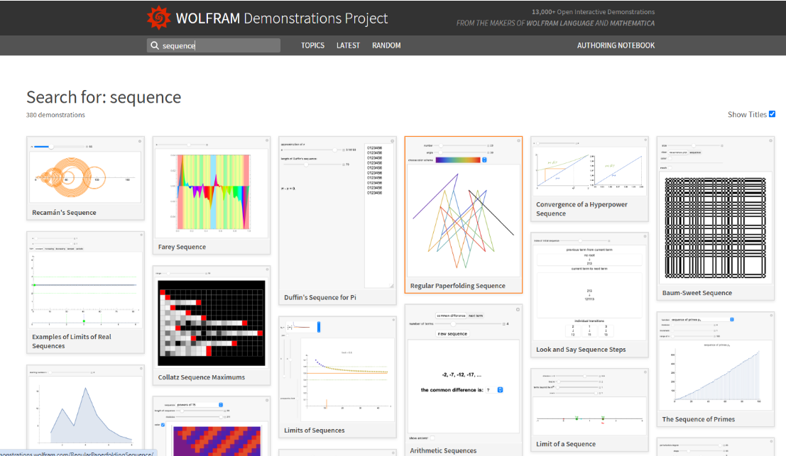
demonstrations.wolfram.com
demonstrations.wolfram.com
Many Demonstrations have sequences.
No-3-in-line problem, A000769
No-3-in-line problem, A000769
In the No-3-in-line problem, no three points are in a line, in any direction.
MathWorld. Uni-bielefeld. Wikipedia.
The number of distinct solutions for n=1, 2, ..., are 1, 1, 4, 5, 11, 22, 57, 51, 156 ... (OEIS A000769).
On 17th June 2026 Marijn Heule used a newly developed SAT solver to find a solution for n=70, a new record.
MathWorld. Uni-bielefeld. Wikipedia.
The number of distinct solutions for n=1, 2, ..., are 1, 1, 4, 5, 11, 22, 57, 51, 156 ... (OEIS A000769).
On 17th June 2026 Marijn Heule used a newly developed SAT solver to find a solution for n=70, a new record.
In[]:=
no3show[s_]:=With[{a=Characters@"0123456789ABCDEFGHIJKLMNOPQRSTUVWXYZabcdefghijklmnopqrstuvwxyz#$%&@?!()[]<>{}=*+|-/~^_:;,.",n=(StringLength[s]-1)/2},With[{p=Join@@MapIndexed[Thread[{#1,n-#2[[1]]}]&,Partition[AssociationThread[a->Range[0,Length[a]-1]]/@Rest@Characters@s,2]]},Graphics[{Thin,Gray,Table[Line[{{0,k},{n,k}}],{k,0,n}],Table[Line[{{k,0},{k,n}}],{k,0,n}],Black,Rectangle[#,#+1]&/@p},AspectRatio->1]]];
This is believed to be the largest solution with full symmetry:
In[]:=
no3show["*45271836090936182745"]
Out[]=
This is the largest known solution with orthogonal mirror symmetry.
In[]:=
no3show["-CFAK7G8JNR3L29EI5P1B06DQMO4H4HMODQ061B5PEI293LNR8J7GAKCF"]
Out[]=
Here’s the largest known solution with double diagonal symmetry:
In[]:=
no3show["xOQAI8N453J3WGOBa2XTV1d7GJKWcXfTb6BVb1L4CCkILek2i06PS0YYgPj9FZe9H5D8EQRUd7jFHDiAZMUEhRhfgNcSaKM"]
Out[]=
A solution for order 65. On June 22, 2026, solutions were also found for orders 67 and 69.
In[]:=
no3show["cgqQm9BVYKoLT6HVgdps#9HK#0U8m4Iac1DswWoPbryNx07ehNS8jF$JTFebx3qvzIk37Cz5ROnZj1nJuafLOv%5f4BRdEW6Ap$QSkyGuY%2ilt2ADPMXlwZhEiUXrtGcCM"]
Out[]=
The largest known solution: order 70, with rotational symmetry. 17 June 2026. Marijn Heule.
In[]:=
no3show["oGYImUVfh6NMux&Vhsy8m6bFWnq5YOP8wT(CJP!MqCT19o%X&dtpt37SX3gnrO?#?Awgku(0DNRBx272jGKR@af#@EIEU4a5Jy!evHl1iov0eBzijZ%HKbsW$Lz9FQc4ADlk$QScdLpZr"]
Out[]=
There are no lines of 3 in any direction:
In[]:=
p70=With[{s="oGYImUVfh6NMux&Vhsy8m6bFWnq5YOP8wT(CJP!MqCT19o%X&dtpt37SX3gnrO?#?Awgku(0DNRBx272jGKR@af#@EIEU4a5Jy!evHl1iov0eBzijZ%HKbsW$Lz9FQc4ADlk$QScdLpZr"},With[{a=Characters@"0123456789ABCDEFGHIJKLMNOPQRSTUVWXYZabcdefghijklmnopqrstuvwxyz#$%&@?!()[]<>{}=*+|-/~^_:;,.",n=(StringLength[s]-1)/2},Join@@MapIndexed[Thread[{#1,n-#2[[1]]}]&,Partition[AssociationThread[a->Range[0,Length[a]-1]]/@Rest@Characters@s,2]]]];
In[]:=
ResourceFunction["FindExtraordinaryLines"][p70]
Out[]=
{}
If we shift mod 35, there are many lines of 3:
In[]:=
shift35=Mod[p70+35,70];three35=ResourceFunction["FindExtraordinaryLines"][shift35];Graphics[{Circle[#,.5]&/@shift35,Thin,Gray,Line[shift35[[#]]]&/@three35}]
What about the other way? Instead of maximal, what’s the minimal?
What’s the minimal number of pieces needed to block 3 in a line?
What’s the minimal number of pieces needed to block 3 in a line?
https://oeis.org/A219760 -- minimize 3-blocking in 2d -- there’s a paper. Martin Gardner's minimum no-3-in-a-line problem.
This is the Queen’s version.
1, 4, 4, 4, 6, 6, 8, 9, 10, 10, 12, 12, 14, 15, 16, 17, 18, 18, 20, 21, 22, 23, 24, 25, 26, 26, 28, 29, 30
https://oeis.org/A277433 is the any slope version:
1, 4, 4, 4, 6, 6, 8, 8, 8, 8
Related: https://oeis.org/A280537 -- no 4 in plane.
This is the Queen’s version.
1, 4, 4, 4, 6, 6, 8, 9, 10, 10, 12, 12, 14, 15, 16, 17, 18, 18, 20, 21, 22, 23, 24, 25, 26, 26, 28, 29, 30
https://oeis.org/A277433 is the any slope version:
1, 4, 4, 4, 6, 6, 8, 8, 8, 8
Related: https://oeis.org/A280537 -- no 4 in plane.
A try for more solutions.
With rotational symmetry
This solution can be moved left or right and still provide coverage.
Here are the coverage lines for order 14.
We can also cover 19x19 with 16 points. I didn’t plan to solve unsolved problems when I started making this talk.
Let’s try for minimal lines with an order 24 solution.
No-3-in-line in 3D (1, 8, 16, 28, 40, 64, ...)
No-3-in-line in 3D (1, 8, 16, 28, 40, 64, ...)
How about 3D? The maximal number of points in an order 3 lattice is 16. Order 4: 28. Order 5: 40. Order 6: 64 Not a sequence, yet.
A003142 Largest subset of 3 X 3 X ... X 3 cube (in n dimensions) with no 3 points collinear. 0, 2, 6, 16, 43, 124, 353
A003142 Largest subset of 3 X 3 X ... X 3 cube (in n dimensions) with no 3 points collinear. 0, 2, 6, 16, 43, 124, 353
No lines of 3:
The next two orders are at least 72 and 88:
History of OEIS
History of OEIS
I use OEIS all the time because it’s useful for solving problems. The typical usage case is:
1. Solve the first five examples.
2. Look it up.
1. Solve the first five examples.
2. Look it up.
1965 Neil Sloane begins collecting integer sequences on file cards, which were later transferred to computer punched cards.
1972 Working at AT&T Bell Labs, Neil Sloane completes the manuscript for the Handbook of Integer Sequences.
1973 A Handbook of Integer Sequences is published, containing 2372 sequences in lexicographic order and assigned N-numbers from 1 to 2372.
1974 Martin Gardner, Mathematical Games (July): “Every recreational mathematician should buy a copy forthwith”.
1996 The original OEIS website (http://www.research.att.com/~njas/sequences/Seis.html) is launched with 10,000 sequences.
2007 NJA Sloane: “I need to get a site. Suggestions?” Me: “oeis.org is available. Buy it.” He did!
More at https://oeis.org/wiki/Timeline_of_the_OEIS
Number of Finite Groups | A000001 | 0, 1, 1, 1, 2, 1, 2, 1, 5, 2, 2, 1, 5, 1, 2, 1, 14, 1, 5, 1, 5, 2, 2, 1, 15
Number of Finite Groups | A000001 | 0, 1, 1, 1, 2, 1, 2, 1, 5, 2, 2, 1, 5, 1, 2, 1, 14, 1, 5, 1, 5, 2, 2, 1, 15
Number of groups of a given order.
A sequence over {1,2} that is equal to its own run-length encoding.
When presented in this form, the term a(n) gives the length of the nth run in the sequence.
When presented in this form, the term a(n) gives the length of the nth run in the sequence.
In[]:=
kolakoski[count_] := Module[{a = {1, 2, 2}, k = 3, value = 1},
While[Length[a] < count,
a = Join[a, ConstantArray[value, a[[k]]]];
value = 3 - value;
k++];
Take[a, count]]
ArrayPlot[Partition[kolakoski[60^2],60]]
While[Length[a] < count,
a = Join[a, ConstantArray[value, a[[k]]]];
value = 3 - value;
k++];
Take[a, count]]
ArrayPlot[Partition[kolakoski[60^2],60]]
Number of divisors | OEIS A000005 | 1, 2, 2, 3, 2, 4, 2, 4, 3, 4, 2, 6, ...
Sum of divisors | OEIS A000203 | 1, 3, 4, 7, 6, 12, 8, 15, 13, 18, 12, 28, ...
Number of divisors | OEIS A000005 | 1, 2, 2, 3, 2, 4, 2, 4, 3, 4, 2, 6, ...
Sum of divisors | OEIS A000203 | 1, 3, 4, 7, 6, 12, 8, 15, 13, 18, 12, 28, ...
Sum of divisors | OEIS A000203 | 1, 3, 4, 7, 6, 12, 8, 15, 13, 18, 12, 28, ...
τ(n), also written d(n), counts the positive divisors of n.
In[]:=
Table[DivisorSigma[0, n], {n, 1, 50}]
Length[Divisors[#]] & /@ Range[50]
Length[Divisors[#]] & /@ Range[50]
σ(n) is the sum of all positive divisors of n. Perfect, abundant and deficient numbers are classified by comparing σ(n)-n with n.
In[]:=
Table[DivisorSigma[1, n], {n, 1, 50}]
Total[Divisors[#]] & /@ Range[50]
Total[Divisors[#]] & /@ Range[50]
Counts integer partitions in which no part is repeated. Equivalently, it counts partitions into odd parts.
In[]:=
Table[ Length @ Select[IntegerPartitions[n], DuplicateFreeQ], {n, 0, 30}]
CoefficientList[Series[Product[1 + x^k, {k, 1, 30}], {x, 0, 30}], x]
CoefficientList[Series[Product[1 + x^k, {k, 1, 30}], {x, 0, 30}], x]
φ(n) counts the positive integers not exceeding n that are coprime to n.
In[]:=
Table[EulerPhi[n], {n, 1, 40}]
Table[Count[Range[n], k_ /; CoprimeQ[k, n]], {n, 1, 20}]
Table[Count[Range[n], k_ /; CoprimeQ[k, n]], {n, 1, 20}]
Counts binary strings of length n up to cyclic rotation.
Counts binary strings up to rotation and reflection. This is the necklace problem with the full dihedral group.
Counts binary strings up to rotation and reflection. This is the necklace problem with the full dihedral group.
In[]:=
necklaceCanonical[{}] = {};
necklaceCanonical[s_] := First @ Sort[
RotateLeft[s, #] & /@ Range[0, Length[s] - 1]]
Table[
Length @ DeleteDuplicates[necklaceCanonical /@ Tuples[{0, 1}, n]],
{n, 0, 12}]
necklaceCanonical[s_] := First @ Sort[
RotateLeft[s, #] & /@ Range[0, Length[s] - 1]]
Table[
Length @ DeleteDuplicates[necklaceCanonical /@ Tuples[{0, 1}, n]],
{n, 0, 12}]
In[]:=
braceletCanonical[{}] = {};
braceletCanonical[s_] := First @ Sort @ Join[
RotateLeft[s, #] & /@ Range[0, Length[s] - 1],
RotateLeft[Reverse[s], #] & /@ Range[0, Length[s] - 1]]
Table[
Length @ DeleteDuplicates[braceletCanonical /@ Tuples[{0, 1}, n]],
{n, 0, 12}]
braceletCanonical[s_] := First @ Sort @ Join[
RotateLeft[s, #] & /@ Range[0, Length[s] - 1],
RotateLeft[Reverse[s], #] & /@ Range[0, Length[s] - 1]]
Table[
Length @ DeleteDuplicates[braceletCanonical /@ Tuples[{0, 1}, n]],
{n, 0, 12}]
Fibonacci's companion sequence, with the same recurrence but different initial conditions.
In[]:=
Table[LucasL[n], {n, 0, 29}]
LinearRecurrence[{1, 1}, {2, 1}, 30]
CoefficientList[Series[(2 - x)/(1 - x - x^2), {x, 0, 29}], x]
LinearRecurrence[{1, 1}, {2, 1}, 30]
CoefficientList[Series[(2 - x)/(1 - x - x^2), {x, 0, 29}], x]
The positive integers with exactly two positive divisors. They are the natural example for sieving, filtering and visual pattern hunting.
In[]:=
Table[Prime[n], {n, 1, 30}]
Select[Range[100], PrimeQ]
Select[Range[100], PrimeQ]
We can make a spiral of points and label them 1, 2, 3 and so on.
Ulam did this in a boring lecture, and then circled the primes. He got a pattern out of it.
Something stranger happens with a hexagonal grid:
Counts the ways to write n as a sum of positive integers, ignoring order.
In[]:=
Table[PartitionsP[n], {n, 0, 30}]
CoefficientList[
Normal @ Series[Product[1/(1 - x^k), {k, 1, 30}], {x, 0, 30}],
x]
CoefficientList[
Normal @ Series[Product[1/(1 - x^k), {k, 1, 30}], {x, 0, 30}],
x]
Here are the partitions for 9.
Let’s show these as stacked columns.
What is the minimal number of horizontal lines needed to represent the partitions of 7?
The classic linear recurrence: each term is the sum of the two previous terms. It also appears in tilings, continued fractions, tree growth and golden-ratio approximations.
In[]:=
Table[Fibonacci[n], {n, 0, 29}]
LinearRecurrence[{1, 1}, {0, 1}, 30]
CoefficientList[Normal @ Series[x/(1 - x - x^2), {x, 0, 29}], x]
LinearRecurrence[{1, 1}, {0, 1}, 30]
CoefficientList[Normal @ Series[x/(1 - x - x^2), {x, 0, 29}], x]
We can get a nice golden spiral out of it.
In binary, the sequence makes an interesting pattern.
In the figure, when viewing reflections, the top row of the checkerboard pattern represents one pane of glass, and the bottom row represents the second pane of glass; reflections can occur on any of the three "surfaces" of the panes.
Each term is the sum of the previous three terms.
In[]:=
LinearRecurrence[{1, 1, 1}, {0, 0, 1}, 30]
CoefficientList[Series[x^2/(1 - x - x^2 - x^3), {x, 0, 29}], x]
CoefficientList[Series[x^2/(1 - x - x^2 - x^3), {x, 0, 29}], x]
Powers of 2 | OEIS A000079 | 1, 2, 4, 8, 16, 32, 64, 128, 256, ...
Powers of 3 | OEIS A000244 | 1, 3, 9, 27, 81, 243, 729, 2187, 6561, ...
Powers of 2 | OEIS A000079 | 1, 2, 4, 8, 16, 32, 64, 128, 256, ...
Powers of 3 | OEIS A000244 | 1, 3, 9, 27, 81, 243, 729, 2187, 6561, ...
Powers of 3 | OEIS A000244 | 1, 3, 9, 27, 81, 243, 729, 2187, 6561, ...
Counts subsets of an n-element set and binary strings of length n.
In[]:=
Table[2^n, {n, 0, 29}]
CoefficientList[Series[1/(1 - 2 x), {x, 0, 29}], x]
Table[n! Coefficient[Series[Exp[2 x], {x, 0, 29}], x^n],{n, 1, 29}]
CoefficientList[Series[1/(1 - 2 x), {x, 0, 29}], x]
Table[n! Coefficient[Series[Exp[2 x], {x, 0, 29}], x^n],{n, 1, 29}]
There are 2^5 subsets of {1,2,3,4,5}
Counts permutations equal to their own inverse; equivalently, permutations made only of fixed points and transpositions.
In[]:=
Table[Sum[n!/(2^k k! (n - 2 k)!), {k, 0, Floor[n/2]}], {n, 0, 15}]
Table[n! Coefficient[Series[Exp[x + x^2/2], {x, 0, 15}], x^n], {n, 1, 15}]
Table[n! Coefficient[Series[Exp[x + x^2/2], {x, 0, 15}], x^n], {n, 1, 15}]
This is an involution. The 9 is in the 1st place and the 1 in in the 9th place.
I made a puzzle out of involutions. https://sudokupad.app/39mhbxagno Every row is an involution.
This is actually an easy puzzle. On the green line, neighboring values differ by 5 or more. Digits do not
repeat on the diagonal.
This is actually an easy puzzle. On the green line, neighboring values differ by 5 or more. Digits do not
repeat on the diagonal.
Counts polyominoes up to translation, rotation and reflection. This is a compact example of generate, canonicalize and deduplicate.
In[]:=
polyNeighbors[p_] := (p + #) & /@ {{1, 0}, {-1, 0}, {0, 1}, {0, -1}}
polyNormalize[pts_] := Module[{mins = Min /@ Transpose[pts]},
Sort[(# - mins) & /@ pts]]
polySymmetries = {
{{1, 0}, {0, 1}}, {{0, -1}, {1, 0}},
{{-1, 0}, {0, -1}}, {{0, 1}, {-1, 0}},
{{-1, 0}, {0, 1}}, {{1, 0}, {0, -1}},
{{0, 1}, {1, 0}}, {{0, -1}, {-1, 0}}};
polyCanonical[pts_] := First @ Sort[
Table[polyNormalize[(m.#) & /@ pts], {m, polySymmetries}]]
freePolyominoes[1] = {{{0, 0}}};
freePolyominoes[n_] := freePolyominoes[n] = DeleteDuplicates[
Flatten[Table[
polyCanonical[Append[p, c]],
{p, freePolyominoes[n - 1]},
{c, Complement[Union @@ (polyNeighbors /@ p), p]}], 1]]
Table[Length[freePolyominoes[n]], {n, 1, 9}]
Counts Dyck paths, balanced parentheses, polygon triangulations, binary trees and many other recursively nested objects.
In[]:=
Table[CatalanNumber[n], {n, 0, 20}]
CoefficientList[
Normal @ Series[(1 - Sqrt[1 - 4 x])/(2 x), {x, 0, 20}],
x]
CoefficientList[
Normal @ Series[(1 - Sqrt[1 - 4 x])/(2 x), {x, 0, 20}],
x]
Counts set partitions: the ways to split n labeled objects into unlabeled nonempty blocks.
In[]:=
Table[Sum[StirlingS2[n, k], {k, 0, n}], {n, 0, 15}]
Counts alternating permutations: up-down or down-up orderings of n labeled objects.
In[]:=
Table[
n! Coefficient[Normal @ Series[Sec[x] + Tan[x], {x, 0, 15}], x^n],
{n, 1, 15}]
n! Coefficient[Normal @ Series[Sec[x] + Tan[x], {x, 0, 15}], x^n],
{n, 1, 15}]
The maximal pieces from n cuts.
A linear recurrence sequence tied to denominators of approximations of Sqrt[2].
In[]:=
LinearRecurrence[{2, 1}, {0, 1}, 30]
CoefficientList[Series[x/(1 - 2 x - x^2), {x, 0, 29}], x]
CoefficientList[Series[x/(1 - 2 x - x^2), {x, 0, 29}], x]
The law of eponymy is that almost everything is named after the wrong person.
Counts permutations of n labeled objects. It is the cleanest example where the exponential generating function is simpler than the ordinary one.
In[]:=
Table[n!, {n, 0, 12}]
Counts permutations with no fixed points: nobody gets their own hat back.
In[]:=
Table[Subfactorial[n], {n, 0, 20}]
Table[
n! Coefficient[Normal @ Series[Exp[-x]/(1 - x), {x, 0, 20}], x^n],
{n, 1, 20}]
Table[
n! Coefficient[Normal @ Series[Exp[-x]/(1 - x), {x, 0, 20}], x^n],
{n, 1, 20}]
Counts ways to place n queens on an n by n chessboard so that none attack each other.
In[]:=
queens[n_] :=
Length @ Select[Permutations[Range[n]],
DuplicateFreeQ[# + Range[n]] && DuplicateFreeQ[# - Range[n]] &]
Table[queens[n], {n, 1, 8}]
Length @ Select[Permutations[Range[n]],
DuplicateFreeQ[# + Range[n]] && DuplicateFreeQ[# - Range[n]] &]
Table[queens[n], {n, 1, 8}]
The dot counts in triangular arrays. A basic finite-difference and ordinary generating-function example.
In[]:=
Table[Binomial[n + 1, 2], {n, 0, 29}]
CoefficientList[Series[x/(1 - x)^3, {x, 0, 29}], x]
CoefficientList[Series[x/(1 - x)^3, {x, 0, 29}], x]
Triangular numbers are integers of the form (n^2+n)/2; they are 0, 1, 3, 6, 10, 15, 21, 28, …. As a teenager, in 1796, Gauss proved that every positive integer can be written as the sum of three or fewer triangular numbers. Jul 10 1796: EYPHKA! num = DELTA + DELTA + DELTA. https://oeis.org/A002636
How many solutions are there?
Numbers of the form 2^n - 1. The prime members are rare and famous.
https://oeis.org/A000043 Mersenne exponents or primes.
In[]:=
Table[2^n - 1, {n, 0, 29}]
CoefficientList[Series[x/((1 - x) (1 - 2 x)), {x, 0, 29}],x]
CoefficientList[Series[x/((1 - x) (1 - 2 x)), {x, 0, 29}],x]
Many Mersenne numbers can be factored.
The most familiar quadratic sequence; its second differences are constant.
In[]:=
Table[n^2, {n, 0, 29}]
CoefficientList[Series[x (1 + x)/(1 - x)^3, {x, 0, 29}], x]
CoefficientList[Series[x (1 + x)/(1 - x)^3, {x, 0, 29}], x]
The three-dimensional analog of triangular numbers: stacked triangular layers.
In[]:=
Table[Binomial[n + 2, 3], {n, 0, 25}]
CoefficientList[Series[x/(1 - x)^4, {x, 0, 25}], x]
CoefficientList[Series[x/(1 - x)^4, {x, 0, 25}], x]
Sums of consecutive squares: the number of balls in a square pyramid.
In[]:=
Table[n (n + 1) (2 n + 1)/6, {n, 0, 20}]
CoefficientList[Series[x (1 + x)/(1 - x)^4, {x, 0, 20}], x]
CoefficientList[Series[x (1 + x)/(1 - x)^4, {x, 0, 20}], x]
Perfect numbers | OEIS A000396 | 6, 28, 496, 8128, 33550336, 8589869056, ...
Abundant numbers | OEIS A005101 | 12, 18, 20, 24, 30, 36, 40, 42, 48, 54, 56, 60, ...
Deficient numbers | OEIS A005100 | 1, 2, 3, 4, 5, 7, 8, 9, 10, 11, 13, 14, ...
Perfect numbers | OEIS A000396 | 6, 28, 496, 8128, 33550336, 8589869056, ...
Abundant numbers | OEIS A005101 | 12, 18, 20, 24, 30, 36, 40, 42, 48, 54, 56, 60, ...
Deficient numbers | OEIS A005100 | 1, 2, 3, 4, 5, 7, 8, 9, 10, 11, 13, 14, ...
Abundant numbers | OEIS A005101 | 12, 18, 20, 24, 30, 36, 40, 42, 48, 54, 56, 60, ...
Deficient numbers | OEIS A005100 | 1, 2, 3, 4, 5, 7, 8, 9, 10, 11, 13, 14, ...
A number is perfect when its proper divisors sum to the number itself. Every known perfect number is even and comes from a Mersenne prime.
In[]:=
mersenneExponents = Select[Range[2, 31], PrimeQ[2^# - 1] &];
(2^(# - 1) (2^# - 1)) & /@ mersenneExponents
Select[Range[10000], DivisorSigma[1, #] == 2 # &]
(2^(# - 1) (2^# - 1)) & /@ mersenneExponents
Select[Range[10000], DivisorSigma[1, #] == 2 # &]
A simple cubic sequence; finite differences make the degree visible.
In[]:=
Table[n^3, {n, 0, 20}]
CoefficientList[Series[x (1 + 4 x + x^2)/(1 - x)^4, {x, 0, 20}], x]
CoefficientList[Series[x (1 + 4 x + x^2)/(1 - x)^4, {x, 0, 20}], x]
Counts weak orderings or preferential arrangements: set partitions whose blocks are ordered.
In[]:=
Table[Sum[k! StirlingS2[n, k], {k, 0, n}], {n, 0, 12}]
Table[ n! Coefficient[Series[1/(2 - Exp[x]), {x, 0, 12}], x^n], {n, 1, 12}]
Table[ n! Coefficient[Series[1/(2 - Exp[x]), {x, 0, 12}], x^n], {n, 1, 12}]
https://mathworld.wolfram.com/CombinationLock.html -- for a door with combination buttons, where more than one button can be pressed at once,
how many combinations are there where each button is pressed once? For 3 buttons, it’s 13.
how many combinations are there where each button is pressed once? For 3 buttons, it’s 13.
OEIS uses the normalization a(0)=1, a(1)=a(2)=0 with a(n)=a(n-2)+a(n-3). The familiar architectural version is a shifted sequence beginning 1,1,1,2,2,3.
In[]:=
LinearRecurrence[{0, 1, 1}, {1, 0, 0}, 30]
CoefficientList[
Normal @ Series[(1 - x^2)/(1 - x^2 - x^3), {x, 0, 29}],
x]
CoefficientList[
Normal @ Series[(1 - x^2)/(1 - x^2 - x^3), {x, 0, 29}],
x]
A positional sieve: begin with the odd numbers, then repeatedly delete every kth surviving number, where k is the next survivor.
In[]:=
lucky[count_] := Module[{a = Range[1, 10000, 2], k = 2, step},
While[k <= Length[a] && Length[a] >= count,
step = a[[k]];
If[step > Length[a], Break[]];
a = Pick[a, Mod[Range[Length[a]], step], Except[0]];
k++];
Take[a, count]]
lucky[30]
While[k <= Length[a] && Length[a] >= count,
step = a[[k]];
If[step > Length[a], Break[]];
a = Pick[a, Mod[Range[Length[a]], step], Except[0]];
k++];
Take[a, count]]
lucky[30]
The move counts for the Chinese rings puzzle. A tiny mechanical puzzle gives a recurrence-like exponential sequence.
In[]:=
Table[Floor[2^(n + 1)/3], {n, 0, 20}]
Counts Motzkin paths: paths from (0,0) to (n,0) using up, down and level steps, never going below the axis. Also counts noncrossing partial matchings.
In[]:=
Table[Hypergeometric2F1[(1 - n)/2, -n/2, 2, 4], {n, 0, 29}]
Table[
Sum[Binomial[n, 2 k] CatalanNumber[k], {k, 0, Floor[n/2]}],
{n, 0, 29}]
Table[
Sum[Binomial[n, 2 k] CatalanNumber[k], {k, 0, Floor[n/2]}],
{n, 0, 29}]
Self-avoiding walks on the square lattice | OEIS A001411 | 1, 4, 12, 36, 100, 284, 780, 2172, 5916, ...
Self-avoiding walks on the square lattice | OEIS A001411 | 1, 4, 12, 36, 100, 284, 780, 2172, 5916, ...
Counts n-step walks from the origin on the square lattice that never visit the same vertex twice.
In[]:=
walkNeighbors[p_] := (p + #) & /@ {{1, 0}, {-1, 0}, {0, 1}, {0, -1}}
walks[0] = {{{0, 0}}};
walks[n_] := walks[n] = Flatten[
Table[
Append[w, p],
{w, walks[n - 1]},
{p, Complement[walkNeighbors[Last[w]], w]}],
1]
Table[Length[walks[n]], {n, 0, 10}]
walks[0] = {{{0, 0}}};
walks[n_] := walks[n] = Flatten[
Table[
Append[w, p],
{w, walks[n - 1]},
{p, Complement[walkNeighbors[Last[w]], w]}],
1]
Table[Length[walks[n]], {n, 0, 10}]
It obeys the same recurrence as the Padovan sequence but has different initial conditions. Perrin divisibility gives a useful probable-prime test.
In[]:=
LinearRecurrence[{0, 1, 1}, {3, 0, 2}, 30]
CoefficientList[Series[(3 - x^2)/(1 - x^2 - x^3), {x, 0, 29}], x]
CoefficientList[Series[(3 - x^2)/(1 - x^2 - x^3), {x, 0, 29}], x]
A central dot surrounded by square layers.
In[]:=
Table[n^2 + (n + 1)^2, {n, 0, 20}]
CoefficientList[Series[(1 + x)^2/(1 - x)^3, {x, 0, 20}], x]
CoefficientList[Series[(1 + x)^2/(1 - x)^3, {x, 0, 20}], x]
Counts lattice paths from (0,0) to (n,n) using horizontal, vertical and diagonal steps.
In[]:=
Table[Sum[Binomial[n, k]^2 2^k, {k, 0, n}], {n, 0, 15}]
CoefficientList[Series[1/Sqrt[1 - 6 x + x^2], {x, 0, 15}],x]
CoefficientList[Series[1/Sqrt[1 - 6 x + x^2], {x, 0, 15}],x]
Products of consecutive integers: n(n+1). Visually, rectangles one unit longer than they are wide.
In[]:=
Table[n (n + 1), {n, 0, 29}]
CoefficientList[Series[2 x/(1 - x)^3, {x, 0, 29}], x]
CoefficientList[Series[2 x/(1 - x)^3, {x, 0, 29}], x]
The area of an oblong is a pronic number. Here are minimal square tilings of oblongs.
The coefficient of x^n in (1 + x + x^2)^n.
In[]:=
Table[Coefficient[(1 + x + x^2)^n, x^n], {n, 1, 20}]
CoefficientList[Series[1/Sqrt[1 - 2 x - 3 x^2], {x, 0, 20}],x]
CoefficientList[Series[1/Sqrt[1 - 2 x - 3 x^2], {x, 0, 20}],x]
Pascal’s tetrahedron of trinomial coefficients reduced modulo k, where k varies between 2 and 11. The colors represent the values of the trinomial coefficients.
A parity-based recurrence whose successive ratios enumerate the positive rational numbers through the Stern-Brocot and Calkin-Wilf trees.
Also called the Fusc sequence.
Also called the Fusc sequence.
Note the numerators and denominators:
Start with 1 and 2. Each new term is the smallest integer having exactly one representation as a sum of two distinct earlier terms.
In[]:=
ulam[count_] := Module[{a = {1, 2}, n = 3},
While[Length[a] < count,
If[Count[Total /@ Subsets[a, {2}], n] == 1, AppendTo[a, n]];
n++];
a]
ulam[30]
While[Length[a] < count,
If[Count[Total /@ Subsets[a, {2}], n] == 1, AppendTo[a, n]];
n++];
a]
ulam[30]
Consecutive terms differ in exactly one bit. It is a Hamiltonian path through the hypercube.
In[]:=
gray = Table[BitXor[n, Quotient[n, 2]], {n, 0, 31}]
Unlike binary, which follows the sequence 000, 001, 010, 011, 100, and so on, a Gray code is one in which only one bit changes between consecutive steps, such as in the sequence 000, 001, 011, 010, 110, and so on. This has many applications, such as reducing the likelihood of reading an incorrect code from encoders. Two types of encoders are shown in this Demonstration, a rotary encoder used to measure rotation, and a linear encoder used to measure absolute distance. The red sensor reads white contacts as zeros and black contacts as ones, so each position of the sensor yields a unique four-digit code. However, if the positions of the contacts on the encoder are anything less than perfect, the sensor might read an incorrect code. Since a Gray code only varies by one bit for consecutive steps, this will never cause the sensor to read a code that is more than one step away from what it should be, which is shown as the “real step” in the Demonstration. Binary has no limit to how many bits can change between steps, so the transition might cause an illogical sequence, such as from steps three to zero to four. The Demonstration shows this by allowing the contacts for one of the bits to become misaligned. If the sensor reads the correct code, the step is displayed in black; if it is one step away, it is displayed in orange; and if it is more than one step away, it is displayed in red.
Integers not divisible by the square of any prime. Equivalently, these are the n for which μ(n) is nonzero.
Select[Range[200], MoebiusMu[#] != 0 &]
At step n, try to subtract n; if that would go negative or hit an old value, add n instead.
In[]:=
recaman[n_] := Module[{a = {0}, t},
Do[
t = Last[a] - k;
AppendTo[a, If[t > 0 && FreeQ[a, t], t, Last[a] + k]],
{k, 1, n}];
a]
recaman[29]
Do[
t = Last[a] - k;
AppendTo[a, If[t > 0 && FreeQ[a, t], t, Last[a] + k]],
{k, 1, n}];
a]
recaman[29]
Each term describes the run lengths of the previous term: one 1, two 1s, one 2 then one 1 and so on.
In[]:=
lookSay[s_] :=
StringJoin[ToString /@ Flatten[{Length[#], First[#]} & /@ Split[Characters[s]]]]
NestList[lookSay, "1", 10]
StringJoin[ToString /@ Flatten[{Length[#], First[#]} & /@ Split[Characters[s]]]]
NestList[lookSay, "1", 10]
The length of the Farey sequence of order n is 1 plus the summatory totient function.
In[]:=
Table[1 + Sum[EulerPhi[k], {k, 1, n}], {n, 0, 30}]
FareySequence[8]
FareySequence[8]
Write the numbers 1 through n in a circle, start at 1 and cross off every other number until only one number is left.
Large Schröder numbers count lattice paths like Catalan paths, but with diagonal steps allowed.
In[]:=
Table[
Sum[Binomial[n + k, 2 k] Binomial[2 k, k]/(k + 1), {k, 0, n}],
{n, 0, 15}]
CoefficientList[
Normal @ Series[(1 - x - Sqrt[1 - 6 x + x^2])/(2 x), {x, 0, 15}],
x]
Sum[Binomial[n + k, 2 k] Binomial[2 k, k]/(k + 1), {k, 0, n}],
{n, 0, 15}]
CoefficientList[
Normal @ Series[(1 - x - Sqrt[1 - 6 x + x^2])/(2 x), {x, 0, 15}],
x]
For each starting value n, count how many 3n+1 steps are needed to reach 1.
In[]:=
collatzStep[n_] := If[EvenQ[n], n/2, 3 n + 1]
collatzLength[n_] :=
Length[NestWhileList[collatzStep, n, # != 1 &]] - 1
Table[collatzLength[n], {n, 1, 30}]
collatzLength[n_] :=
Length[NestWhileList[collatzStep, n, # != 1 &]] - 1
Table[collatzLength[n], {n, 1, 30}]
The binomial coefficients read by rows. A single triangular array contains powers of 2, triangular numbers, Fibonacci diagonals and the mod-2 Sierpinski gasket.
The signed Stirling triangle gives coefficients of falling factorials. Absolute values count permutations by number of cycles.
In[]:=
Table[StirlingS1[n, k], {n, 1, 8}, {k, 1, n}]
Flatten @ Table[StirlingS1[n, k], {n, 1, 8}, {k, 1, n}]
Flatten @ Table[StirlingS1[n, k], {n, 1, 8}, {k, 1, n}]
Counts partitions of an n-element set into k nonempty blocks. Bell numbers are the row sums.
In[]:=
Table[StirlingS2[n, k], {n, 1, 8}, {k, 1, n}]
Total /@ Table[StirlingS2[n, k], {n, 1, 10}, {k, 1, n}]
Total /@ Table[StirlingS2[n, k], {n, 1, 10}, {k, 1, n}]
The Eulerian triangle counts permutations according to their number of ascents or descents.
μ(n) is zero when n has a squared prime factor; otherwise its sign records the parity of the number of prime factors.
In[]:=
Table[MoebiusMu[n], {n, 1, 50}]
The parity of the number of 1s in the binary expansion of n. It is also generated by the substitution 0→01, 1→10.
In[]:=
Table[Mod[DigitCount[n, 2, 1], 2], {n, 0, 31}]
Nest[Join[#, 1 - #] &, {0}, 5]
Nest[Join[#, 1 - #] &, {0}, 5]
The left-right turn sequence obtained by repeatedly folding a strip of paper. It is a classic automatic sequence connected with the dragon curve.
Table[ Boole[Mod[(n + 1)/2^IntegerExponent[n + 1, 2], 4] == 1], {n, 0, 31}]
Counts cyclic binary sequences in which every binary string of length n occurs exactly once.
In[]:=
Table[2^(2^(n - 1) - n), {n, 1, 8}]
In groups of 5, all the combinations are covered.
It becomes more obvious when the partitions are sorted.
For n>0, the term is 1 exactly when every block of consecutive zeros in the binary expansion of n has even length.
In[]:=
baumSweet[0] = 0;
baumSweet[n_Integer?Positive] := Boole[
AllTrue[
StringLength /@ StringCases[IntegerString[n, 2], RegularExpression["0+"]],
EvenQ]]
Table[baumSweet[n], {n, 0, 31}]
baumSweet[n_Integer?Positive] := Boole[
AllTrue[
StringLength /@ StringCases[IntegerString[n, 2], RegularExpression["0+"]],
EvenQ]]
Table[baumSweet[n], {n, 0, 31}]
Mondrian Art Problem | OEIS A276523 | 2, 4, 4, 5, 5, 6, 6, 8, 6, 7, 8, 6, 8, 8, 8, 8, 8, 9, 9, 9, 8, 9
Mondrian Art Problem | OEIS A276523 | 2, 4, 4, 5, 5, 6, 6, 8, 6, 7, 8, 6, 8, 8, 8, 8, 8, 9, 9, 9, 8, 9
Partition an n X n square into multiple non-congruent integer-sided rectangles. a(n) is the least possible difference between the largest and smallest area.
Unsolved
Unsolved
Some of the best known solutions for Martin Gardner’s minimal no-3-in-a-line problem, all slopes version. https://oeis.org/A277433
CITE THIS NOTEBOOK
CITE THIS NOTEBOOK
Mathematical Games: integer sequences
by Ed Pegg
Wolfram Community, STAFF PICKS, June 25, 2026
https://community.wolfram.com/groups/-/m/t/3739534
by Ed Pegg
Wolfram Community, STAFF PICKS, June 25, 2026
https://community.wolfram.com/groups/-/m/t/3739534