This project builds a simplified “airspace” cellular automaton for studying congestion under time-varying capacity. Aircraft are modeled as conserved load moving across a grid of sectors via simple local routing preferences toward destination boundaries. A moving storm field reduces sector service capacity, creating transient and persistent bottlenecks that induce queueing, spillback, and throughput oscillations: emergent phenomena that arise without any global path planning. Through animations of raw load and utilization as well as time-series of throughput and system occupancy, the notebook illustrates how local rules and local constraints can produce realistic macroscopic traffic patterns, and how multi-destination flows interact to form and compete over dominant corridors.
Introduction
Introduction
Air traffic flow management must balance stochastic demand with limited airspace capacity that varies over time due to weather, sector workload, and operational constraints. High-fidelity simulators and optimization-based methods can be accurate but are often complex, expensive to run, and less visually transparent. At the opposite extreme, purely conceptual models can be interpretable but may not produce measurable emergent behavior.
This project aims to bridge that gap with an applied-math–friendly approach: a cellular automaton for airspace flow that is (i) simple enough to implement and experiment with quickly, (ii) rich enough to produce realistic macroscopic phenomena like congestion waves and spillback, and (iii) compatible with quantitative evaluation and “control-like” interventions. The key idea is to treat the airspace as a lattice of sectors that exchange load locally each tick, under capacity constraints that are endogenously modulated by weather. The result is a tractable dynamical system where global behavior (e.g., throughput, delay, queue growth) emerges from local rules.
This project aims to bridge that gap with an applied-math–friendly approach: a cellular automaton for airspace flow that is (i) simple enough to implement and experiment with quickly, (ii) rich enough to produce realistic macroscopic phenomena like congestion waves and spillback, and (iii) compatible with quantitative evaluation and “control-like” interventions. The key idea is to treat the airspace as a lattice of sectors that exchange load locally each tick, under capacity constraints that are endogenously modulated by weather. The result is a tractable dynamical system where global behavior (e.g., throughput, delay, queue growth) emerges from local rules.
Baseline Model: One Origin to One Sink
Baseline Model: One Origin to One Sink
Model at a Glance
Model at a Glance
State. Each cell is an airspace sector. The state variable (i,j)≥0 is the number (or density) of aircraft in that sector at tick . A moving storm induces a weather severity field (i,j)∈[0,1] that lowers capacity.
Capacities. Weather-adjusted service is(i,j)(1-α(i,j)). Each sector also has a finite buffer (i,j) limiting how much inflow it can accept in one tick.
Update idea. Each tick: (1) demand enters at the west boundary, (2) each sector proposes sending some of its load to neighbors using a local preference (progress east, detour around bad weather / congestion), and (3) receiving sectors scale/clip inflows to respect buffer/capacity. This single “acceptance scaling” step is what produces queueing and spillback.
(i,j)
L
t
t
W
t
Capacities. Weather-adjusted service is
C
t
C
0
W
t
B
t
Update idea. Each tick: (1) demand enters at the west boundary, (2) each sector proposes sending some of its load to neighbors using a local preference (progress east, detour around bad weather / congestion), and (3) receiving sectors scale/clip inflows to respect buffer/capacity. This single “acceptance scaling” step is what produces queueing and spillback.
State and Interpretation
State and Interpretation
The simulator is a macroscopic airspace cellular automaton defined on an grid of sectors. The main state variable is the sector load (i,j)≥0, which represents the number (or density) of aircraft currently occupying sector at tick . In code, is stored as numeric matrix. The full simulator state is a pair {,}, where storm_t is a small record containing the storm’s center location (and any auxiliary motion parameters). Each tick updates both components: the storm moves stochastically, generating a new weather field (i,j), and then the load is advanced via local flow and capacity constraints.
We initialize the airspace empty (0 everywhere) and place the storm center near the middle of the grid. Demand enters from the west boundary (left side): at each tick, we inject Poisson arrivals into a fixed set of sourceRows. This is the simplest “airport-like” entry model: aircraft appear at the boundary, then propagate through the sector network subject to downstream capacity limits.
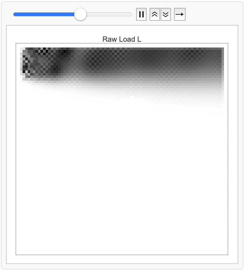
The plot below visualizes the raw sector load as a heatmap (darker = higher load). At this early stage, almost all nonzero load appears in the leftmost column, because the only mechanism that has acted so far is demand injection at the west boundary. The small vertical band of dark pixels corresponds exactly to the designated source rows: those are the sectors that received newly injected aircraft during this tick. The remainder of the grid is still empty because the injected mass has not yet propagated far into the interior.
nn
L
t
(i,j)
t
L
t
state
t
L
t
storm
t
W
t
L
t
We initialize the airspace empty (
L
0
The plot below visualizes the raw sector load
L
t

Figure (Raw load ). Darker cells indicate higher aircraft density. The storm creates a reduced-capacity region; upstream of it, load thickens as spillback forms, while downstream the grid “drains” and becomes lighter.
L
t
Weather-Driven Capacity and the Moving Storm
Weather-Driven Capacity and the Moving Storm
We now visualize how the sector load field (i,j) evolves over time when demand enters from the west boundary and a moving storm locally reduces capacity: each tick, aircraft enter along a fixed set of source rows (a vertical “entry band” on the left). These arrivals then propagate through the grid via local movement rules that favor eastward progress, with a smaller probability of lateral (north/south) diversion.
As time progresses, the injected mass forms an advecting “plume” that moves east across the grid. The main structure in this run is a dominant high-density corridor in the upper portion of the airspace. This is not hard-coded as a route; it emerges from the combination of (i) where demand enters (source rows), (ii) directional bias in the local routing rule, and (iii) downstream constraints. The visible checker/texture early in the run is a consequence of discrete, stochastic injection (Poisson arrivals) and the fact that load is updated in local, per-cell transactions.
A key feature of the animation is the appearance of a large low-load/empty region in the center shaped like a disk/semidisk. This corresponds to the storm’s weather footprint: weather increases(i,j), which reduces sector capacity (i,j) (and, in our implementation, effectively limits how much load can pass through or accumulate in that region). As the east-moving flow reaches this reduced-capacity area, the model’s acceptance/buffering constraints cause upstream buildup and rerouting around the footprint. Visually, this shows up as (1) a thickening/darkening of load upstream of the bottleneck and (2) a “shadow” region where the storm suppresses throughput.
L
t
As time progresses, the injected mass forms an advecting “plume” that moves east across the grid. The main structure in this run is a dominant high-density corridor in the upper portion of the airspace. This is not hard-coded as a route; it emerges from the combination of (i) where demand enters (source rows), (ii) directional bias in the local routing rule, and (iii) downstream constraints. The visible checker/texture early in the run is a consequence of discrete, stochastic injection (Poisson arrivals) and the fact that load is updated in local, per-cell transactions.
A key feature of the animation is the appearance of a large low-load/empty region in the center shaped like a disk/semidisk. This corresponds to the storm’s weather footprint: weather increases
W
t
C
t
Out[]=
Raw load (i,j) is useful for seeing where aircraft accumulate, but it can be misleading when capacity is heterogeneous: a sector with load might be uncongested if its capacity is , but critically overloaded in . To make sure congestion comparable across the grid, we visualize the utilization (or saturation) ratio (i,j)(i,j)(i,j). Here (i,j) is the weather-adjusted per-tick capacity, computed from the storm-induced severity field (i,j) via (i,j)(1-α(i,j)). In other words, the same weather footprint that creates a “hole” in the raw load animation also creates a region of sharply reduced capacity; makes the bottleneck explicit.In the visualization, the large red disk corresponds to the storm footprint where is high and is low. Even if the raw load inside/near the storm is not extremely large, dividing by a small yields a high utilization: this region is operating near (or beyond) its processing limit and becomes the dominant constraint on system throughput. Outside the storm, the ratio is much lighter because capacity is higher; sectors can absorb and forward traffic without saturating. This plot therefore diagnoses where the system is truly capacity-constrained, not just where aircraft happen to be present. The simulation is at the top of the notebook.
L
t
L3
C10
C2
R
t
L
t
C
t
C
t
W
t
C
t
C
0
W
t
R
t
W
t
C
t
C
t

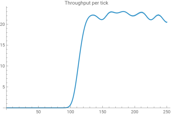
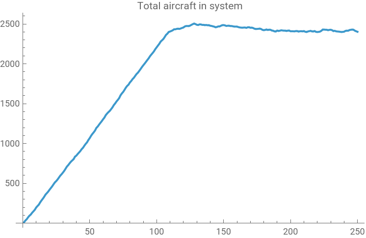
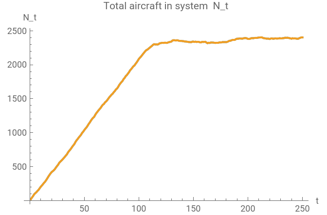
Even though the dynamics are implemented as local CA updates, the grid behaves like a stochastic flow network with a conserved “mass.” Let (i,j)≥0 be the aircraft load in sector at tick , and define total occupancy (i,j). Each tick injects new aircraft at entry sectors, transports load through the interior under capacity/buffer constraints, and removes aircraft that reach the sink boundary. If is the number of injected arrivals and is the number that exit (throughput), then the simulation approximately satisfies the mass balance +-, (up to clipping from buffer enforcement). Inflow is Poisson on sourceRows west-boundary rows; with rate 𝜆 per row, . For and , , giving a natural steady-state target ≈ when the network is stable.The long initial period where ≈0 is a finite travel-time effect: aircraft must cross the grid before any can exit. With lateral bias , the eastward preference in the update is ≈1-2b; here , so a crude crossing-time estimate is ≈≈≈114 ticks, which matches the observed “warm-up” before throughput ramps. After this transient, the dominant source of variability is the moving storm: weather severity (i,j)∈[0,1] reduces sector capacity via (i,j)(1-α(i,j)), so as the storm drifts across (or near) the main corridor, the effective service rate of the network fluctuates. That shows up macroscopically as oscillations in and a high plateau: i.e., a persistent backlog whose level reflects congestion induced by time-varying capacity.
L
t
(i,j)
t
N
t
n
∑
i1
n
∑
j1
L
t
A
t
Q
t
N
t+1
N
t
A
t
Q
t
E[]λ·sourceRows
A
t
λ1.8
sourceRows12
E[]≡21.6
A
t
Q
A
Q
t
blateralBias
w
E
b0.15⇒≈0.7
w
E
t
travel
n
w
E
80
0.7
W
t
C
t
C
0
W
t
Q
t
N
t
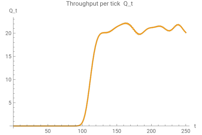
To confirm that the congestion patterns are genuinely weather-driven (and not an artifact of the routing rule), I run a matched pair of simulations with identical demand and routing settings. In the control run, weather is disabled by setting the storm-capacity coupling to zero (), while keeping everything else the same.
To make the comparison fair, I reuse the same random seed in both runs so that the Poisson arrivals (and, if the simulator draws storm motion from the same RNG stream) are matched. With no weather impact, throughput ramps after the travel-time transient and stabilizes near the injection rate. With weather enabled, throughput dips whenever the storm footprint intersects a dominant corridor, and the system accumulates a persistent backlog.
α0
To make the comparison fair, I reuse the same random seed in both runs so that the Poisson arrivals (and, if the simulator draws storm motion from the same RNG stream) are matched. With no weather impact, throughput ramps after the travel-time transient and stabilizes near the injection rate. With weather enabled, throughput dips whenever the storm footprint intersects a dominant corridor, and the system accumulates a persistent backlog
N
t
Multi-Airport Multi-Destination Variant
Multi-Airport Multi-Destination Variant
Up to this point, the simulator treated all aircraft as interchangeable. To get something closer to “air traffic,” I added a multi-airport, multi-destination variant where aircraft carry a destination label. Concretely, the scalar load field (i,j) becomes a stack of commodity fields (i,j)≥0, k1,...,K, one per destination airport, and the total sector load is the sum Demand is now specified by an OD matrix : each origin airport injects Poisson arrivals destined for each , so the mix of traffic entering the system is heterogeneous from the start.The key modeling choice is how “destination intent” appears without global path planning. In the update rule, each commodity proposes moves using a soft preference toward its destination: neighboring sectors that reduce distance-to-go are favored, while neighbors with worse weather or high congestion are penalized. A simple way to express this is a one-step “cost-to-go” for each candidate move, followed by a softmax:
L
t
K
(k)
L
t
Conclusion and Future Directions
Conclusion and Future Directions
We implemented a cellular automaton model of airspace flow that demonstrates how congestion phenomena emerge from simple local routing rules under time-varying capacity constraints. The model successfully reproduces realistic traffic patterns including spillback, throughput oscillations, and corridor formation without requiring global path planning or optimization. Through visualizations of raw load, normalized utilization, and time-series analysis, we showed that a moving weather field creates persistent bottlenecks that induce queueing behavior characteristic of real air traffic networks. The multi-destination extension revealed how commodity-specific routing preferences interact to form competing corridors under shared capacity constraints. Future work could incorporate the modeling of strategic rerouting based on weather forecasts and control interventions such as ground delay programs or dynamic sector reconfigurations. Calibrating the model against real traffic data from database feeds would enable validation and establish whether emergent patterns match observed congestion in actual airspace.
References
References
◼
Bilimoria, K. D., Sridhar, B., Chatterji, G. B., Sheth, K. S., & Grabbe, S. (2016). FACET: Future ATM Concepts Evaluation Tool. Air Traffic Control Quarterly, 9(1), 1–20. DOI: https://doi.org/10.2514/atcq.9.1.1
◼
Ball, M. O., Barnhart, C., Dresner, M., Hansen, M., Neels, K., Odoni, A., Peterson, E., Sherry, L., Trani, A., & Zou, B. (2010). Total Delay Impact Study: A Comprehensive Assessment of the Costs and Impacts of Flight Delay in the United States. NEXTOR. LINK: https://rosap.ntl.bts.gov/view/dot/6234
◼
Nagel, K., Schreckenberg, M. (1992). A Cellular Automaton Model for Freeway Traffic. Journal de Physique Archives, 2(12), 2221–2229. DOI: https://doi.org/10.1051/jp1:1992277
◼
Due to upload size restrictions, I have taken a screenshot of my interactive simulations and put them in as jpgs. If you would like my full simulations, I have included a google drive link: https://drive.google.com/drive/folders/1ZP5LiE8S-AU7BaoMm5UERplD6jKhcN4p?usp=sharing. Here is the full code for the notebook: https://drive.google.com/file/d/1ENslTnAbKszYwIcxrA4iPkdGTPWrcZnf/view
CITE THIS NOTEBOOK
CITE THIS NOTEBOOK
A cellular automaton airspace: emergent congestion from local routing under moving weather
by Guhan Thiagarajan
Wolfram Community, STAFF PICKS, February 3, 2026
https://community.wolfram.com/groups/-/m/t/3632429
by Guhan Thiagarajan
Wolfram Community, STAFF PICKS, February 3, 2026
https://community.wolfram.com/groups/-/m/t/3632429