Expressions of Isothermal Effectiveness Factor using Symbolic Computations
Authors: Housam Binous, André Von-Held Soares, Fernando Cunha Peixoto, Ahmed Bellagi
Expressions of Isothermal Effectiveness Factor using Symbolic Computations
Authors: Housam Binous, André Von-Held Soares, Fernando Cunha Peixoto, Ahmed Bellagi
Authors: Housam Binous, André Von-Held Soares, Fernando Cunha Peixoto, Ahmed Bellagi
References:
1- L. D. Schmidt, The Engineering of Chemical Reactions, Oxford University Press, 1998.
2- H. S. Fogler, Elements of Chemical Reaction Engineering, 3rd Edition, Prentice Hall, 1999.
3- O. Levenspiel, Chemical Reaction Engineering, 3rd Edition, Wiley 1999.
1- L. D. Schmidt, The Engineering of Chemical Reactions, Oxford University Press, 1998.
2- H. S. Fogler, Elements of Chemical Reaction Engineering, 3rd Edition, Prentice Hall, 1999.
3- O. Levenspiel, Chemical Reaction Engineering, 3rd Edition, Wiley 1999.
Porous Catalyst Slab
Porous Catalyst Slab
Solving differential equation resulting from shell balance and using boundary conditions: CA'[0]=0 and CA[l]=CAs with =
2
λ
'''
k
D
e
In[]:=
sol1=DSolve[D[CA[x],{x,2}]λ^2CA[x],CA[x],x]
Out[]=
CA[x]+
xλ
1
-xλ
2
In[]:=
CA[x_]:=C1+C2
-xλ
xλ
In[]:=
sol2=Solve[{CA'[0]0,CA[l]CAs},{C1,C2}]
Out[]=
C1,C2
CAs
lλ
1+
2lλ
CAs
lλ
1+
2lλ
In[]:=
C1=sol2[[1,1,2]]
Out[]=
CAs
lλ
1+
2lλ
In[]:=
C2=sol2[[1,2,2]]
Out[]=
CAs
lλ
1+
2lλ
In[]:=
CA[x]/.(Cosh[2lλ]+Sinh[2lλ])/.(Cosh[lλ-xλ]+Sinh[lλ-xλ])/.(Cosh[lλ+xλ]+Sinh[lλ+xλ])//Simplify
2lλ
lλ-xλ
lλ+xλ
Out[]=
CAsCosh[xλ]Sech[lλ]
Computing the effectiveness factor
In[]:=
η=Integrate[CAsCosh[xλ]Sech[lλ],{x,0,l}]/(lCAs)
Out[]=
Tanh[lλ]
lλ
In[]:=
η=/.λϕ/l
Tanh[lλ]
lλ
Out[]=
Tanh[ϕ]
ϕ
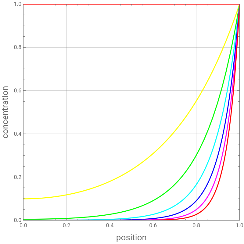
Plotting concentration profile for different values of λ when CAs=1 and l=1.
Whenis large (λ is small):
CA is close to CAs over most of the catalyst particle. There is no resistance to pore diffusion limitation and expect η to be close to unity.
Whenis small (λ is large):
CA is close to zero over most of the catalyst particle, there are strong pore diffusion effects and expect η to be small compared to one.
When
D
e
CA is close to CAs over most of the catalyst particle. There is no resistance to pore diffusion limitation and expect η to be close to unity.
When
D
e
CA is close to zero over most of the catalyst particle, there are strong pore diffusion effects and expect η to be small compared to one.
In[]:=
l=1;CAs=1;
In[]:=
CA[x]//Simplify
Out[]=
λ-xλ
λ+xλ
1+
2λ
In[]:=
Plot[Evaluate[Table[CA[x],{λ,0,20,3}]],{x,0,1},PlotStyleTable[Hue[λ/30],{λ,0,30,5}],PlotRange{{0,1},{0,1}},Frame->True,GridLines->Automatic,AspectRatio->1,ImageSize->400{1,1},FrameLabel{Style["position",14],Style["concentration",14]},PlotLegends->Table[λ,{λ,0,20,3}]]
Out[]=


In[]:=
l=.;CAs=.;
Porous Catalyst Spheres
Porous Catalyst Spheres
Solving differential equation resulting from shell balance and using boundary conditions: CA finite at r=0 and CA[R0]=CAs with =
2
λ
'''
k
D
e
In[]:=
CA[x_]=.;
In[]:=
C1=.;C2=.;
In[]:=
sol3=DSolve[1/r^2D[r^2D[CA[r],{r,1}],{r,1}]λ^2CA[r],CA[r],r]//Factor
Out[]=
CA[r]2λ+
-rλ
1
2rλ
2
2rλ
In[]:=
CA[r_]:=(2λC1+C2)
-rλ
2rλ
2rλ
2 λ C1+ C2=0 because CA must be finite at r=0
In[]:=
Solve[2λC1+C2==0,C1]
Out[]=
C1-
C2
2λ
In[]:=
C1=-;
C2
2λ
In[]:=
sol4=Solve[CA[R0]CAs,C2]//Simplify
Out[]=
C2
2CAsR0λ
R0λ
-1+
2R0λ
In[]:=
C2=sol4[[1,1,2]]
Out[]=
2CAsR0λ
R0λ
-1+
2R0λ
In[]:=
CA[r]/.(Cosh[-rλ]+Sinh[-rλ])/.(Cosh[2rλ]+Sinh[2rλ])//FullSimplify
-rλ
2rλ
Out[]=
CAsR0Csch[R0λ]Sinh[rλ]
r
Computing the effectiveness factor
In[]:=
η=Integrate4Pir^2,{r,0,R0}(4Pi/3R0^3CAs)//Simplify
CAsR0Csch[R0λ]Sinh[rλ]
r
Out[]=
3(-1+R0λCoth[R0λ])
2
R0
2
λ
In[]:=
η=/.λϕ/R0
3(-1+R0λCoth[R0λ])
2
R0
2
λ
Out[]=
3(-1+ϕCoth[ϕ])
2
ϕ
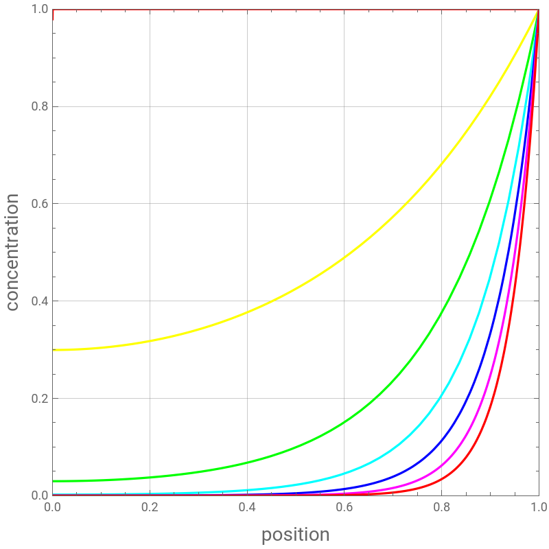
Plotting concentration profile for different values of λ when CAs=1 and l=1.
Whenis large (λ is small):
CA is close to CAs over most of the catalyst particle. There is no resistance to pore diffusion limitation and expect η to be close to unity.
Whenis small (λ is large):
CA is close to zero over most of the catalyst particle, there are strong pore diffusion effects and expect η to be small compared to one.
When
D
e
CA is close to CAs over most of the catalyst particle. There is no resistance to pore diffusion limitation and expect η to be close to unity.
When
D
e
CA is close to zero over most of the catalyst particle, there are strong pore diffusion effects and expect η to be small compared to one.
In[]:=
R0=1;CAs=1;
In[]:=
Plot[Evaluate[Table[CA[x],{λ,0.0000001,20,3}]],{x,0,1},PlotStyleTable[Hue[λ/30],{λ,0,30,5}],PlotRange{{0,1},{0,1}},Frame->True,GridLines->Automatic,AspectRatio->1,ImageSize->400{1,1},FrameLabel{Style["position",14],Style["concentration",14]},PlotLegends->Table[λ,{λ,0,20,3}]]
Out[]=
Porous Catalyst Cylinders
Porous Catalyst Cylinders
C2=0 because CA must be finite at r=0
Computing the effectiveness factor
Effectiveness factor versus Thiele modulus for porous particles of various shapes.
Effectiveness factor versus Thiele modulus for porous particles of various shapes.
Same plot is given in Ref . 3