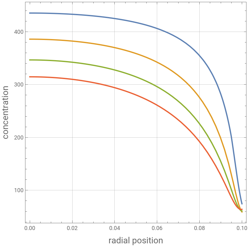
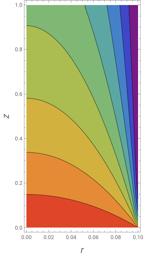
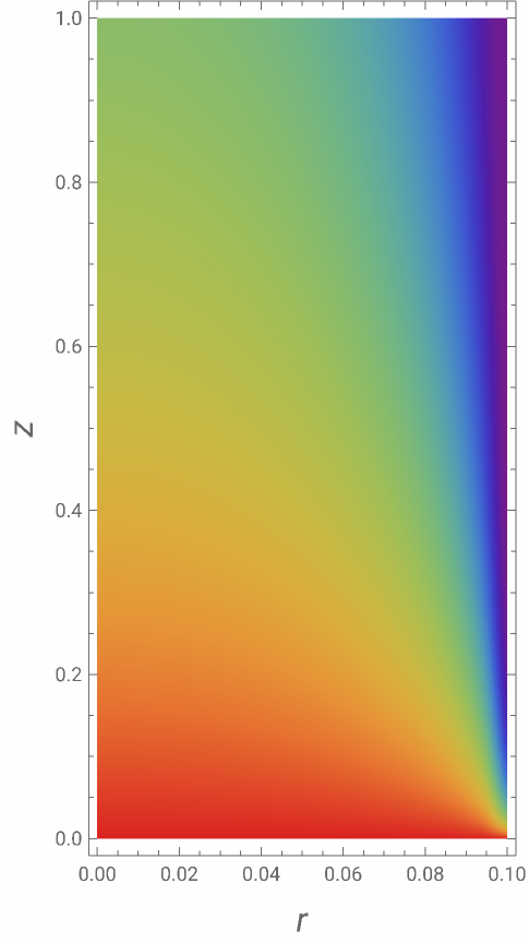
We plot Figure 4 of Ref . 2, which gives the concentration in a laminar flow reactor (Newtonian fluid case) versus the radial position for selected values of the axial position . We also draw contour and density plots. Finally, the value of the mixing cup concentration is computed. Here, the solution is based on the finite difference method.
Values of the parameters obtained from Fogler’s COMSOL-ECRE see Ref. 1
Uk=1300;Cpc=4180;mc=0.01;k=0.559;DH=-83680;Dp=10^-9;Ea=95238;A=1.110^8;rho=1000;Cp=4180;U=v0/(PiR^2);Rg=8.314;v0=510^-4;Ta0=298;Keq0=1000;rhocat=1500;T0=320;Ca0=500;R=0.1;L=1.0;Nr=40;Nz=40;
Positions of the nodes - we adopt a uniform grid
rgrid=R/NrRange[0,Nr];zgrid=L/NzRange[0,Nz];
Concentrations
values=Outer[Ca,rgrid,zgrid];
Partial derivative operators
L1r=NDSolve`FiniteDifferenceDerivative[Derivative[1,0],{rgrid,zgrid},values,"DifferenceOrder"8];L2r=NDSolve`FiniteDifferenceDerivative[Derivative[2,0],{rgrid,zgrid},values,"DifferenceOrder"8];L1z=NDSolve`FiniteDifferenceDerivative[Derivative[0,1],{rgrid,zgrid},values,"DifferenceOrder"8];L2z=NDSolve`FiniteDifferenceDerivative[Derivative[0,2],{rgrid,zgrid},values,"DifferenceOrder"8];
Governing equations
Eq1[i_,j_]:=Dp1/rgrid[[i]]L1r[[i,j]]+DpL2r[[i,j]]+DpL2z[[i,j]]-2U(1-(rgrid[[i]]/R)^2)L1z[[i,j]]+ra[i,j]0;
Conversions
xa=1-values/Ca0;
Rate equation
ra[i_,j_]:=-AExp[-Ea/(RgT0)]rhocat(values[[i,j]]^2-1/(Keq0Exp[DH/Rg(1/303-1/T0)])(2Ca0xa[[i,j]])^2)
Boundary conditions
BC1=Table[values[[i,1]]Ca0,{i,1,Nr+1}];BC2=Table[L1r[[1,j]]0,{j,2,Nz}];BC3=Table[L1r[[Nr+1,j]]0,{j,2,Nz}];BC4=Table[L1z[[i,Nz+1]]0,{i,1,Nr+1}];
Unknown concentrations
unknowns=Join[Flatten[Table[{values[[i,j]],300},{i,1,Nr+1},{j,1,Nz+1}],1]];
System of equations to be solved using FindRoot
sys=Flatten[Join[{BC1,BC2,BC3,BC4,Flatten[Table[Eq1[i,j],{i,2,Nr},{j,2,Nz}],1]}],1];
sol=FindRoot[sys,unknowns,MaxIterations1000];
Plotting the concentration profiles at different axial positions - we reproduce Fig. 4 of Ref. 2
a=Flatten[Table[{rgrid[[i]],zgrid[[j]],values[[i,j]]/.sol},{i,1,Nr+1},{j,1,Nz+1}],1];f=Interpolation[a,InterpolationOrder3]P1=Plot[{f[x,0.2],f[x,0.4],f[x,0.6],f[x,0.8]},{x,0,0.1},FrameTrue,GridLinesAutomatic,PlotStyleThick,AspectRatio1,ImageSize400{1,1},PlotLegends{"z=0.2","z=0.4","z=0.6","z=0.8"},FrameLabel{Style["radial position",14],Style["concentration",14]}]
Out[]=
InterpolatingFunction


Out[]=


Contour plot of concentration
ContourPlot[f[x,y],{x,0,0.1},{y,0,1},PlotPoints200,FrameLabel{Style["r",Italic,16],Style["z",Italic,16]},PlotLegendsAutomatic,ColorFunction"Rainbow",PlotRangeAll,AspectRatio2]
Out[]=

Density plot of concentration
DensityPlot[f[x,y],{x,0,0.1},{y,0,1},PlotPoints200,FrameLabel{Style["r",Italic,16],Style["z",Italic,16]},PlotLegendsAutomatic,ColorFunction"Rainbow",PlotRangeAll,AspectRatio2]
Out[]=

Computation of mixing-cup concentration
NIntegrate[2Pi2Ur(1-(r/R)^2)f[r,1],{r,0,0.1}]/NIntegrate[2Pi2Ur(1-(r/R)^2),{r,0,0.1}]
Out[]=
231.701
References
References
◼
◼
[2] A.-H. Soares, L. de Sousa Santos, H. Binous, A. A. Shaikh, and A. Bellagi, Exploring tubular steady-state laminar flow reactors with orthogonal collocation, Comput. Appl. Eng. Educ. (2024), e22795. https://doi.org/10.1002/cae.22795
CITE THIS NOTEBOOK
CITE THIS NOTEBOOK
Fogler's isothermal laminar flow reactor solved using the finite difference method
by André von-Held Soares, Lizandro de Sousa Santos, Housam Binous, Abdullah A. Shaikh and Ahmed Bellagi
Wolfram Community, STAFF PICKS, September 14, 2024
https://community.wolfram.com/groups/-/m/t/3273933
by André von-Held Soares, Lizandro de Sousa Santos, Housam Binous, Abdullah A. Shaikh and Ahmed Bellagi
Wolfram Community, STAFF PICKS, September 14, 2024
https://community.wolfram.com/groups/-/m/t/3273933