Wolfram Cloud Document

Diffusion tensor imaging based fiber tractography
by Martijn Froeling

Introduction

The nuclear magnetic resonance signal can be made dependant on the diffusion of the water in tissue as was first shown by Steskal and Tanner [1]. When magnetic resonance imaging was developed it was le Bihan et al. who in the 80s showed that diffusion weighed images could be acquired [2]. The diffusion weighted signal in tissue is directional dependant and when measured in multiple directions the diffusion signal can be described using a 2nd order tensor as was first described by Basser et al. in the 90s [3-4]. This method is now knows as diffusion tensor imaging, or DTI. The tensor can be decomposed in its eigensystem where the eigenvectors are the principal diffusion directions of the tissue and the eigenvalues the diffusion magnitude. The principal eigenvector points in the principal direction of anisotropic tissue e.g. neurons or muscle cells. This method is called fiber tractography and was first proposed by Mori et al. in the 90s [5].This If one traces the principal eigenvectors using streamlines a representation of the underlying tissue architecture can be made.

[1] Stejskal, E. O., & Tanner, J. E. (1965). Spin diffusion measurements: Spin echoes in the presence of a time-dependent field gradient. The Journal of Chemical Physics, 42(1), 288–292. https://doi.org/10.1063/1.1695690
[2] Le Bihan, D., Breton, E., Lallemand, D., Grenier, P., Cabanis, E., & Laval-Jeantet, M. (1986). MR imaging of intravoxel incoherent motions: application to diffusion and perfusion in neurologic disorders. Radiology, 161(2), 401–407. https://doi.org/10.1148/radiology.161.2.3763909
[3] Basser, P. J., Mattiello, J., & Lebihan, D. (1994). Estimation of the Effective Self-Diffusion Tensor from the NMR Spin Echo. Journal of Magnetic Resonance, Series B, 103(3), 247–254. https://doi.org/10.1006/jmrb.1994.1037
[4] Mattiello, J., Basser, P. J., & Le Bihan, D. (1997). The b matrix in diffusion tensor echo-planar imaging. Magnetic Resonance in Medicine, 37(2), 292–300. https://doi.org/10.1002/mrm.1910370226
[5] Mori, S., Crain, B. J., Chacko, V. P., & Van Zijl, P. C. M. (1999). Three-dimensional tracking of axonal projections in the brain by magnetic resonance imaging. Annals of Neurology, 45(2), 265–269. https://doi.org/10.1002/1531-8249(199902)45:2<265::AID-ANA21>3.0.CO;2-3

The math

The diffusion weighed signal can be described as

(

) =



with

the diffusion tensor,

x,i

y,i

z,i

the diffusion weighting direction,

the diffusion weighting strength,

the unweighted MRI signal and

(

) the diffusion weighted signal. This equation can be rewritten as

(

) =



with



x,i

y,i

z,i

-2

x,i

y,i

-2

z,i

x,i

-2

z,i

y,i



and



Ln(

)



.If at least 7 measurements with at least 2 different b-values are done one can solve the system

Ln



such that for each location the diffusion tensor is known.

The Data

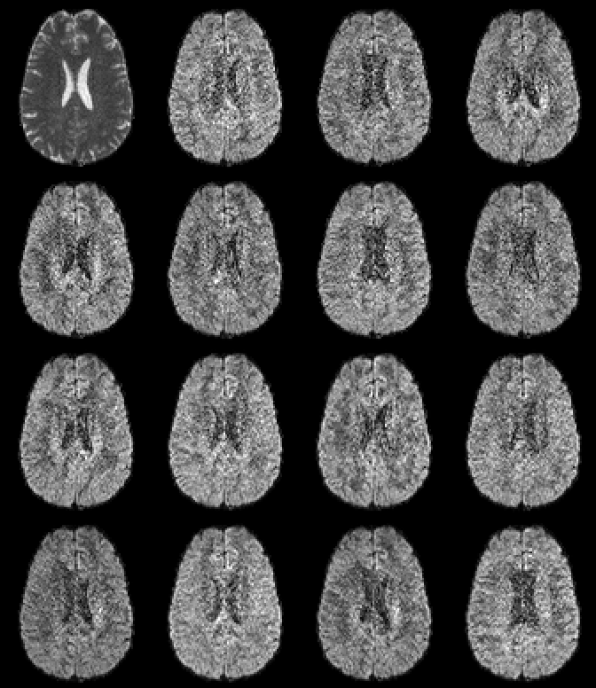
Diffusion weighted images of a brain look like this (images are rescaled, the diffusion weighted images contain much lower signal). Typical datasets are 60x128x128 voxels with between 40 to 150 volumes (different combinations of g and b).

The Tensor

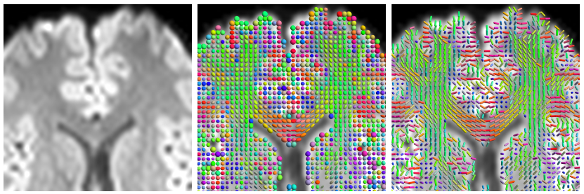
For each location in the data the tensor can be fitted and represented by an ellipsoid or a stick representing the principal eigen vector. We used standard color coding where red is left-rigth, green is front-back, and blue is up-down.

Tractography

Fiber tractography of the principal eigen vectors generates a tachogram. There are many software tools that can do this, but i wanted to add this to my toolbox in Mathematica, just because its fun to do and could be useful in the future.

Tractography is done from a seed point from where the vector field is followed using a defined step size. Since the vector field is bi-directional the tensors are interpolated and the eigenvectors calculated for the new location. Tractography is stopped when a stop criteria is met of the tracts propagate with an angle above a certain thresh hold. Propagation can be done using Euler or Runge-Kutta methods.

The Code

Options[FiberTractography]={FiberLengthRange->{10,200},FiberAngle->30,SeedSpacing->2,SeedRandomization->0.5,TensorFilps->{1,1,1},TensorPermutations->{"x","y","z"},InterpolationOrder->1,StopThreshhold->0.5,StepSize->2,Method->"Euler"};

FiberTractography[tensor_,vox_,opts:OptionsPattern[]]:=(Print[0];FiberTractography[tensor,vox,{1,{0,1}},opts])FiberTractography[tensor_,vox_,{par_?ArrayQ,{min_?NumberQ,max_?NumberQ}},opts:OptionsPattern[]]:=FiberTractography[tensor,vox,{{par,{min,max}}},opts]

FiberTractography[tensor_,vox_,inp:{{_,{_,_}}...},opts:OptionsPattern[]]:=Block[{lmin,lmax,amax,seedSp,seedRand,flip,per,int,stopT,step,tensTr,voxTr,inpTr,treshs,coors,ran,stop,intE,intS,intF,drop,sx,sy,sz,ex,ey,ez,seeds,tracts,iii,t1},(*gettheoptions*){lmin,lmax}=OptionValue[FiberLengthRange];amax=OptionValue[FiberAngle];seedSp=OptionValue[SeedSpacing];seedRand=Clip[OptionValue[SeedRandomization],{0,1}];flip=OptionValue[TensorFilps];per=OptionValue[TensorPermutations];int=OptionValue[InterpolationOrder];stopT=OptionValue[StopThreshhold];step=OptionValue[StepSize];intF=Switch[OptionValue[Method],"RungeKutta",RK2,"RungeKutta4",RK4,_,Euler];(*preparedata*)tensTr=FlipTensorOrientation[TransData[#,"l"]&/@tensor,{"y","x","z"},{1,1,1}];voxTr=RotateLeft[vox,1];(*convertdimensionsofstoppings*){inpTr,treshs}=Transpose[inp];inpTr=Transpose[{TransData[#,"l"]&/@inpTr,treshs}];(*getthedatacoordinatesoncenterofvoxels*)coors=Flatten[Array[vox{#1,#2,#3}-0.5vox&,Dimensions[tensTr][[2;;]]],2];(*createstoppingmask*)stop=Unitize[Mean[Abs[tensTr[[1;;3]]]]](Times@@(Mask[#[[1]],#[[2]]]&/@inpTr));(*makethetracandstopinterpolationfunctions*)intE=Interpolation[Thread[{coors,Flatten[TransData[tensTr,"l"],2]}],InterpolationOrderint];intS=Interpolation[Thread[{coors,Flatten[stop,2]}],InterpolationOrderint];(*maketheseedpoint*){sx,sy,sz}=0.5vox;{ex,ey,ez}=voxDimensions[tensTr][[2;;]]-0.5vox;seeds=Flatten[Table[{x,y,z},{x,sx,ex,seedSp},{y,sy,ey,seedSp},{z,sz,ez,seedSp}],2];seeds=seeds+RandomReal[NormalDistribution[0,seedRand],Dimensions[seeds]];seeds=Quiet@Pick[seeds,UnitStep[(intS@@Transpose[seeds])-0.5],1];Print["number of seedpoints: ",Length[seeds]];t1=First[AbsoluteTiming[tracts=Monitor[Table[TractFunc[seeds[[iii]],step,{amax,lmax,stopT},{intE,intS,intF}],{iii,1,Length[seeds]}],ProgressIndicator[iii,{0,Length[seeds]}]];tracts=If[stepLength[#]>lmax,drop=Ceiling[(stepLength[#]-lmax)/(2step)]+1;#[[drop;;-drop]],#]&/@Select[tracts,lmin<stepLength[#]&];]];Print["Tractography took ",t1," seconds"];Print[Length[tracts]," tracts were generated with average length ",stepRound[Mean[Length/@tracts],.1],"mm"];tracts]

Introduction

The math

The Data

The Tensor

Tractography

The Code

Performing tractography