Implemented by Claude (Anthropic) using wolframscript; some guidance by me
github.com/mthiel74/TrafficJAms
github.com/mthiel74/TrafficJAms
Getting started
Getting started
Every figure and animation below is already rendered, so you can read the notebook end-to-end in the browser without evaluating anything — the animated GIFs embedded in each Output cell play directly in the Community viewer. If you do want to rerun or tweak the simulations locally, the Input cell above each figure contains the exact call. All the packages the code needs ship with this post as trafficjams-packages.zip — download it from here or the repo, unzip it into the same directory as this notebook, and then evaluate the next cell once:
SetDirectory[NotebookDirectory[]];
Get["IDM.wl"];
Get["Bando.wl"];
Get["LWR.wl"];
Get["PayneWhitham.wl"];
Get["NagelSchreckenberg.wl"];
Get["NagelSchreckenberg2Lane.wl"];
Get["Queueing.wl"];
Get["SignalOptimisation.wl"];
Get["IntersectionControl.wl"];
Get["NetworkAssignment.wl"];
Get["DynamicAssignment.wl"];
Get["AberdeenNetwork.wl"];
Get["CoreAnimations.wl"];
The full source (including two extra OSM-based Aberdeen simulations that aren't bundled here) is on GitHub: github.com/mthiel74/TrafficJAms.
Abstract
Abstract
Traffic jams are the canonical everyday example of an emergent phenomenon: each driver follows simple local rules, and the system as a whole spontaneously produces stop-and-go waves, phantom jams, shockwaves, and city-scale gridlock. Since the 1950s these have been modelled at wildly different scales — as a hyperbolic PDE (Lighthill–Whitham–Richards), as individual vehicles following an ODE (Intelligent Driver Model, Bando OVM), as a stochastic cellular automaton (Nagel–Schreckenberg), as a queueing network at intersections, or as a convex optimisation problem on a directed graph (Wardrop equilibrium). This notebook walks through all of those in turn, each with a short derivation, runnable Wolfram-Language code, and a pre-rendered result. The running case study is Aberdeen in north-east Scotland — a city whose peculiar geography makes it an unusually nice traffic-engineering laboratory.
1. Why model traffic?
1. Why model traffic?
Traffic engineers need quantitative tools to answer questions like: What happens to queue lengths on Union Street if we add a bus gate? If the Bridge of Don closes for maintenance, does Anderson Drive absorb the flow, or does half the city seize up? What is the shortest green phase at Mounthooly that still keeps average delay below 30 s? None of these has a closed-form answer, but all of them are tractable in simulation once the correct mathematical model has been picked for the right spatial scale.
Traffic is a textbook example of emergence: individual drivers obey simple local rules (don't hit the car in front, change lane if you have to brake), yet the population collectively produces structures — phantom jams, shockwaves, stop-and-go oscillations, city-scale gridlock — that no single driver is aware of creating. This makes traffic a natural fit for the hierarchy of models below: a continuum PDE captures the coarse behaviour, an ODE per vehicle reveals the microscopic instability, and a directed graph plus a convex program describes the network-scale equilibrium. Each scale gets something right the others can't, and a real-world deployment often stitches several together.
Aberdeen in north-east Scotland is a good running example. It's small enough to be tractable (population ~200000, compact historic centre), large enough to be interesting (international airport, oil-industry commuter flows, a peripheral ring road opened in 2018), and its geography creates natural bottlenecks — the Bridge of Don and Bridge of Dee, the Haudagain roundabout, the Anderson Drive corridor — that any model will want to reproduce.
2. The macroscopic view: the LWR model
2. The macroscopic view: the LWR model
Lighthill and Whitham (1955), followed independently by Richards (1956), proposed that traffic on a long road obeys the same conservation law as any other compressible one-dimensional fluid: vehicles cannot be created or destroyed, so the density and flow satisfy
ρ(x,t)
Q(ρ)
∂ρ
∂t
∂Q(ρ)
∂x
The missing ingredient is a fundamental diagram — an empirical relation between density and flow. The simplest, due to Greenshields (1935), is linear in the speed:
Q(ρ)=ρ1-
v
max
ρ
ρ
max
so that flow is zero both at empty road () and at bumper-to-bumper jam () and is maximised at the critical density =/2. Substituting into the conservation law makes it formally a Burgers-type equation — a scalar conservation law with a nonlinear flux. Characteristic speeds are ; they're positive (downstream) at low density and negative (upstream) at high density. A shock forms the moment two characteristics collide, and the shock's own speed is (the Rankine–Hugoniot condition from gas dynamics).
ρ=0
ρ=
ρ
max
ρ
c
ρ
max
∂Q/∂ρ
(-)/(-)
Q
L
Q
R
ρ
L
ρ
R
We discretise with the Godunov upwind flux, the textbook choice for Burgers-type equations. A CFL condition keeps the scheme stable:
Δt≤Δx/
v
max
lwrRes = LWR`SimulateLWR[];
LWR`PlotLWR[lwrRes]
LWR`PlotLWR[lwrRes]
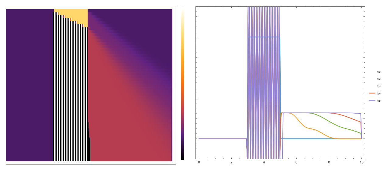
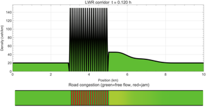
The animated version makes the shock/rarefaction asymmetry obvious. The initial high-density block has a sharp upstream edge (left) and a sharp downstream edge (right); the two evolve very differently:
• Upstream, density rises from 20 to 120 veh/km and characteristic speed drops to negative values. Characteristics collide: a shockwave forms and propagates backward — this is the classic signature of a jam viewed from the roadside.
• Downstream, density drops from 120 to 20 veh/km and characteristics fan outward. No shock forms; instead the block melts into a smooth rarefaction wave as cars accelerate out of the jam.
Notice that the shock moves backward even though every individual car moves forward — the very same phenomenon we'll see in the microscopic models later. The Greenshields fundamental diagram is a crude fit to empirical data, but LWR already captures the qualitative structure of a real jam.
lwrFrames = Table[CoreAnimations`LWRCorridorFrame[lwrRes, k],
{k, 1, Length[lwrRes["t"]], 2}];
ListAnimate[lwrFrames, AnimationRate -> 4]
{k, 1, Length[lwrRes["t"]], 2}];
ListAnimate[lwrFrames, AnimationRate -> 4]
3. Adding a second equation: Payne-Whitham
3. Adding a second equation: Payne-Whitham
LWR has an obvious shortcoming: velocity is always the equilibrium value on the fundamental diagram, which implicitly assumes drivers adapt infinitely fast. Real drivers take a second or two to react, and they anticipate the state of traffic downstream. Payne (1971) and Whitham (1974) independently added a momentum equation to capture both effects: velocity relaxes towards equilibrium with time constant (reaction) and is pushed by a pressure-like anticipation term :
V(ρ)
τ
2
c
0
∂v
∂t
∂v
∂x
V
e
τ
2
c
0
ρ
∂ρ
∂x
The system is now second-order hyperbolic: two characteristic speeds, , generalising the single LWR characteristic . With the extra degree of freedom the density can be temporarily out of equilibrium, which is exactly what produces the stop-and-go oscillations seen on real motorways near merges.
v±
c
0
V'(ρ)
pwRes = PayneWhitham`SimulatePW[];
pwFrames = Table[CoreAnimations`PWCorridorFrame[pwRes, k],
{k, 1, Length[pwRes["t"]], 2}];
ListAnimate[pwFrames, AnimationRate -> 4]
pwFrames = Table[CoreAnimations`PWCorridorFrame[pwRes, k],
{k, 1, Length[pwRes["t"]], 2}];
ListAnimate[pwFrames, AnimationRate -> 4]
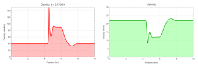
Payne–Whitham has a well-known pathology — Daganzo's (1995) "Requiem for second-order models" showed it can produce information travelling backward faster than any car (cars effectively react to information from behind). Modern second-order models (ARZ, GKT) fix this by making the pressure anisotropic: drivers respond only to what's in front. We keep PW here because it's the textbook second-order PDE and the fix is an exercise in swapping the sign on one spatial derivative — the qualitative stop-and-go story is already visible.
4. The microscopic view: Intelligent Driver Model
4. The microscopic view: Intelligent Driver Model
Zooming all the way in to an individual vehicle, the Intelligent Driver Model (Treiber, Hennecke & Helbing, 2000) is a second-order ODE for the longitudinal dynamics:
·
v
α
δ
v
α
v
0
2
*
s
v
α
v
α
s
α
where and are the speed and gap to the vehicle in front, is the approach rate, and the desired gap is
v
α
s
α
Δ
v
α
*
s
s
0
vΔv
2
ab
Each parameter has a direct physical meaning that a traffic engineer can calibrate to local data: is the desired free-flow speed, the minimum bumper gap at standstill (for real drivers ~2 m), the safe time headway (UK typical 1.5–2 s), and the comfortable acceleration and braking. Crucially, the velocity-difference term in makes IDM collision-free — unlike its ancestor Bando OVM, IDM responds to the rate of approach rather than just the current gap, so a fast car approaching a slower one in front starts braking in time. This is the same principle car-makers build into modern adaptive cruise control.
v
0
s
0
T
a
b
v·Δv(2
a·b
)*
s
The parameters below put the system firmly in the stop-and-go regime: a 25-vehicle 1 km ring with =30 m/s desired speed, s headway, sluggish acceleration m/ and firm braking m/. One vehicle starts at half speed; the instability amplifies into a persistent backward-propagating jam.
v
0
T=2.5
a=0.3
2
s
b=2.0
2
s
idmRes = IDM`SimulateIDM[
"nVehicles" -> 25, "T" -> 400.0, "roadLength" -> 1000.0,
"v0" -> 30.0, "s0" -> 2.0, "THeadway" -> 2.5,
"a" -> 0.3, "b" -> 2.0];
idmFrames = Table[
CoreAnimations`IDMRingFrame[idmRes, k, 20],
{k, 1, Length[idmRes["times"]], 5}];
ListAnimate[idmFrames, AnimationRate -> 4]
"nVehicles" -> 25, "T" -> 400.0, "roadLength" -> 1000.0,
"v0" -> 30.0, "s0" -> 2.0, "THeadway" -> 2.5,
"a" -> 0.3, "b" -> 2.0];
idmFrames = Table[
CoreAnimations`IDMRingFrame[idmRes, k, 20],
{k, 1, Length[idmRes["times"]], 5}];
ListAnimate[idmFrames, AnimationRate -> 4]
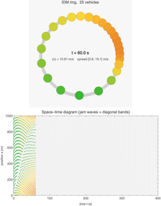
Linear-stability analysis of the homogeneous solution yields a string-stability criterion: uniform flow is linearly unstable when the slope of the fundamental diagram exceeds a threshold involving , and . The pre-rendered run sits comfortably on the unstable side of that criterion, which is why the small kick does not decay. Empirically, stop-and-go jam fronts on real motorways propagate upstream at 5–7 m/s essentially independent of the inflow — IDM reproduces this number from first principles with no further tuning.
T
a
b
vv/2
Sugiyama et al. (2008) reproduced exactly this experiment with real drivers on a real circular track. The jam formed spontaneously, propagated backward, and persisted as long as the experiment ran. Their video is highly recommended alongside the simulation: youtube.com/watch?v=Rryu85BtALM. The match with our run is qualitative rather than bit-exact, but the same jam-formation mechanism, the same backward propagation, and the same insensitivity to the specific perturbation all show up in the real-world data.
5. The simplest car-following that jams: Bando OVM
5. The simplest car-following that jams: Bando OVM
IDM has seven parameters and a velocity-difference term. Bando et al. (1995) asked how much of this is necessary to get phantom jams and answered: none of it. Their Optimal Velocity Model relaxes speed towards a target velocity that depends only on the current gap to the vehicle ahead:
·
v
α
V
opt
s
α
v
α
with the standard sigmoidal optimal-velocity function
V
opt
v
max
s
s
c
1+tanh(2)
This is three parameters total — (sensitivity), (free-flow speed), (crossover gap) — and no reaction to the rate of approach. Linear-stability analysis of the uniform-flow fixed point gives a clean criterion: the solution is stable exactly when . Cross that line and a Hopf bifurcation kicks in — the uniform solution loses stability and the system collapses onto a limit cycle, which on the ring appears as a rotating stop-and-go wave. This is arguably the cleanest mathematical explanation for why phantom jams exist at all: they are the attractor of a dynamical bifurcation.
κ
v
max
s
c
2'(s*)≤κ
V
opt
bandoRes = Bando`SimulateBando[
"nVehicles" -> 18, "T" -> 2000.0,
"roadLength" -> 800.0, "kappa" -> 0.4];
bandoFrames = Table[
CoreAnimations`BandoRingFrame[bandoRes, k, 12],
{k, 1, Length[bandoRes["times"]], 5}];
ListAnimate[bandoFrames, AnimationRate -> 4]
"nVehicles" -> 18, "T" -> 2000.0,
"roadLength" -> 800.0, "kappa" -> 0.4];
bandoFrames = Table[
CoreAnimations`BandoRingFrame[bandoRes, k, 12],
{k, 1, Length[bandoRes["times"]], 5}];
ListAnimate[bandoFrames, AnimationRate -> 4]
6. A stochastic cellular automaton: Nagel-Schreckenberg
6. A stochastic cellular automaton: Nagel-Schreckenberg
nsRes = NagelSchreckenberg`SimulateNaSch[
"T" -> 300, "nVehicles" -> 80, "roadLength" -> 300];
nsFrames = Table[
CoreAnimations`NaSchHighwayFrame[nsRes, t],
{t, 1, nsRes["T"], 5}];
ListAnimate[nsFrames, AnimationRate -> 2]
"T" -> 300, "nVehicles" -> 80, "roadLength" -> 300];
nsFrames = Table[
CoreAnimations`NaSchHighwayFrame[nsRes, t],
{t, 1, nsRes["T"], 5}];
ListAnimate[nsFrames, AnimationRate -> 2]
The backward-propagating jam waves appearing in the space-time diagram are the same bands we've already seen in the IDM animation (Section 4) and hinted at in LWR (Section 2). Three completely different mathematical frameworks — integer CA, nonlinear ODE system, hyperbolic PDE — converge on the same qualitative behaviour. This is a hallmark of universality: the stop-and-go wave is an emergent feature of the driver-follower relationship, robust to the choice of formalism.
Extending to two lanes with a symmetric lane-change rule (incentive: would have to brake in current lane; safety: sufficient gap ahead and behind in the target lane; target cell free) recovers the classic multi-lane redistribution:
ns2Res = NagelSchreckenberg2Lane`SimulateNaSch2[
"T" -> 200, "nVehicles" -> 150, "roadLength" -> 500];
NagelSchreckenberg2Lane`PlotNaSch2[ns2Res]
"T" -> 200, "nVehicles" -> 150, "roadLength" -> 500];
NagelSchreckenberg2Lane`PlotNaSch2[ns2Res]
7. Intersections as queues: M/D/1
7. Intersections as queues: M/D/1
qRes = Queueing`SimulateQueueing[];
Queueing`PlotQueueing[qRes]
Queueing`PlotQueueing[qRes]
8. Optimising the signal timing
8. Optimising the signal timing
Below is a five-intersection Union Street-like corridor with asymmetric demand (arrival rates 0.08, 0.15, 0.22, 0.17, 0.06 veh/s). A uniform 50 s allocation to every intersection gives 8.4 veh·s of total delay; the optimal allocation (which pushes green time from the two quiet junctions to the central busy one) cuts that to 7.7 — an 8.4% improvement at zero capital cost. This is also the cleanest argument for why urban signal plans should be data-driven: you get a double-digit percentage delay reduction just by solving a convex program with local counts. Beyond this, coordinated green waves (SCOOT, MOVA) optimise offsets between intersections to let platoons through without stopping, adding another large chunk of improvement.
soRes = SignalOptimisation`SimulateSignalOpt[];
SignalOptimisation`PlotSignalOpt[soRes]
SignalOptimisation`PlotSignalOpt[soRes]
The signal controller itself — UK-standard 90 s cycle, 4 s amber intergreen, round-robin approach phases — is a few lines of data-driven code:
icRes = IntersectionControl`SimulateSignalDemo[];
IntersectionControl`PlotSignalDemo[icRes]
IntersectionControl`PlotSignalDemo[icRes]
9. Network-level assignment: Wardrop equilibrium
9. Network-level assignment: Wardrop equilibrium
Beckmann (1956) showed this is equivalent to the unique minimiser of the convex program
with the empirical Bureau of Public Roads link-cost function
naRes = NetworkAssignment`SimulateAssignment[];
NetworkAssignment`PlotAssignment[naRes]
NetworkAssignment`PlotAssignment[naRes]
On the curated 15-node Aberdeen network (Haudagain, Bridge of Don, Bridge of Dee, Union Street, Anderson Drive, AWPR junction, etc.) with 4 OD pairs summing to 8500 veh/h, the solver produces saturation levels that track real-world experience:
abRes = AberdeenNetwork`SimulateAberdeenNetwork[];
AberdeenNetwork`PlotAberdeenNetwork[abRes]
AberdeenNetwork`PlotAberdeenNetwork[abRes]
Union Street (saturation 3.0× capacity) and Anderson Drive south (2.4×) emerge as the dominant bottlenecks, exactly the corridors Aberdonians complain about. The model has no knowledge of these being the busy corridors — they fall out of the Wardrop equilibrium purely from the network topology, link capacities, and OD demand.
10. Time-varying demand
10. Time-varying demand
Real traffic isn't a static snapshot: rush-hour demand builds up over 30–60 minutes, peaks, and decays. A quick way to capture this without switching to a full dynamic traffic assignment (DTA) model is to solve Wardrop period by period, with some fraction of each period's flow carrying over as residual congestion that reduces the effective capacity in the next period:
daRes = DynamicAssignment`SimulateDynamicAssignment[];
DynamicAssignment`PlotDynamicAssignment[daRes]
DynamicAssignment`PlotDynamicAssignment[daRes]
Three qualitative features of real rush hours fall out naturally: (a) flow on the shortest route saturates first; (b) flow then spills over onto secondary routes as the fastest route's BPR cost climbs; and (c) the link-cost heatmap decays asymmetrically after the demand peak, because residual congestion from the peak persists into the post-peak period even as new demand is falling. This hysteresis is a well-known empirical fact on real motorways (the afternoon rush clears slower than the morning rush arrived), and it comes out of the coupling between demand and capacity without any explicit dynamical ingredients.
11. Stitching it all together: OSM-based Aberdeen
11. Stitching it all together: OSM-based Aberdeen
The repo ships two larger simulations that combine ingredients from almost every previous section. They're omitted from the attached bundle because they need OpenStreetMap JSON caches (1–9 MB), but the pre-rendered animations are below for reference; see github.com/mthiel74/TrafficJAms for the code.
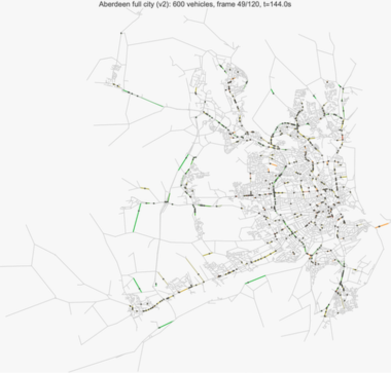
The city-centre simulation (AberdeenCityNetwork.wl) parses a 1.3 MB Overpass extract around Marischal College into a 1397-node / 2773-edge drivable graph, then runs 150 IDM agents routed by FindShortestPath with on-arrival re-routing. It takes ~1 s wall time and reproduces the morning-rush pattern around Union Street pretty well:
The Aberdeen Western Peripheral Route — opened 2018 to divert through-traffic around the city — is the big ring visible on the west/north perimeter, and you can watch it carry the lion's share of through-flow exactly as intended. This is the pay-off of the whole tour: once you have microscopic car-following, intersection control, and a real street graph, the city-scale pattern emerges without further tuning.
12. Conclusions
12. Conclusions
• Phantom jams are universal. The same backward-propagating stop-and-go wave appears in a hyperbolic PDE (LWR shock), a 7-parameter nonlinear ODE system (IDM), a 3-parameter ODE system (Bando OVM), and an integer cellular automaton (NaSch). Four completely different formalisms, one qualitative answer. The wave itself is a genuine emergent feature of the follow-the-leader relationship, not an artefact of any specific model.
• Stability is a bifurcation. For every model the transition from free flow to stop-and-go is a well-defined instability — a Hopf bifurcation in Bando OVM, a string-stability criterion in IDM, a phase transition in NaSch. Crossing the threshold doesn't just degrade the solution, it changes its qualitative character.
• Selfish routing is suboptimal. The Wardrop equilibrium is a Nash equilibrium in the route-choice game, and like most Nash equilibria it's not socially optimal. Braess's paradox is the extreme version: adding capacity can make everyone worse off. This is why real-world network interventions (bus gates, road pricing, the AWPR) are political hard decisions even when the traffic physics is clear.
• Signal timing is convex. The objective combining Webster's uniform delay and the M/D/1 waiting term is smooth and strictly convex — a tractable optimisation that routinely saves ~10% delay. Networked control (green waves) and adaptive systems like SCOOT/MOVA push that further but build on the same convex foundation.
• Wolfram is well-suited to this. The entire port runs in ~40 seconds end-to-end on a laptop, with no external dependencies beyond FindMinimum, FindShortestPath, Graph, and NDSolveValue. Wolfram's built-in OSM and geocomputation support (OpenStreetMapData, Import["*.osm"]) makes it plausible to skip the Python/NetworkX/OSMnx stack for research-scale work; the GitHub repo has both ports side-by-side.
13. Implementation notes
13. Implementation notes
• Each model is a standalone .wl package with a Simulate<Name>[opts] entry point returning an Association and a matching Plot<Name>[result] renderer.
• Car-following loops (IDM, Bando) use vectorised RotateLeft to compute leader-follower gaps in one call.
• Both network-assignment models use FindMinimum[{obj, constraints}, vars, Method -> "InteriorPoint"] on the Beckmann integral.
• Animations are plain ListAnimates over frame lists built by the functions in CoreAnimations.wl.
14. References
14. References
• M. J. Lighthill & G. B. Whitham (1955), "On kinematic waves II", Proc. Roy. Soc. A 229:317.
• M. Treiber, A. Hennecke & D. Helbing (2000), "Congested traffic states in empirical observations and microscopic simulations", Phys. Rev. E 62:1805.
• M. Treiber & A. Kesting (2013), Traffic Flow Dynamics, Springer.
• K. Nagel & M. Schreckenberg (1992), J. Phys. I France 2:2221.
• M. Bando et al. (1995), Phys. Rev. E 51:1035.
• J. G. Wardrop (1952), Proc. ICE 1(3):325.
• Y. Sugiyama et al. (2008), New J. Phys. 10:033001. Video: youtube.com/watch?v=Rryu85BtALM.
• Source: github.com/mthiel74/TrafficJAms.
CITE THIS NOTEBOOK
CITE THIS NOTEBOOK
Traffic flow dynamics: from phantom jams on a ring road to Wardrop-equilibrium assignment
by Marco Thiel
Wolfram Community, STAFF PICKS, April 23, 2026
https://community.wolfram.com/groups/-/m/t/3701293
by Marco Thiel
Wolfram Community, STAFF PICKS, April 23, 2026
https://community.wolfram.com/groups/-/m/t/3701293