The ternary liquid–liquid equilibrium (LLE) of the aniline–hexane–methylcyclopentane system at 45 °C was calculated using the NRTL activity-coefficient model through two independent numerical approaches: the common tangent method and the arc-length continuation method.
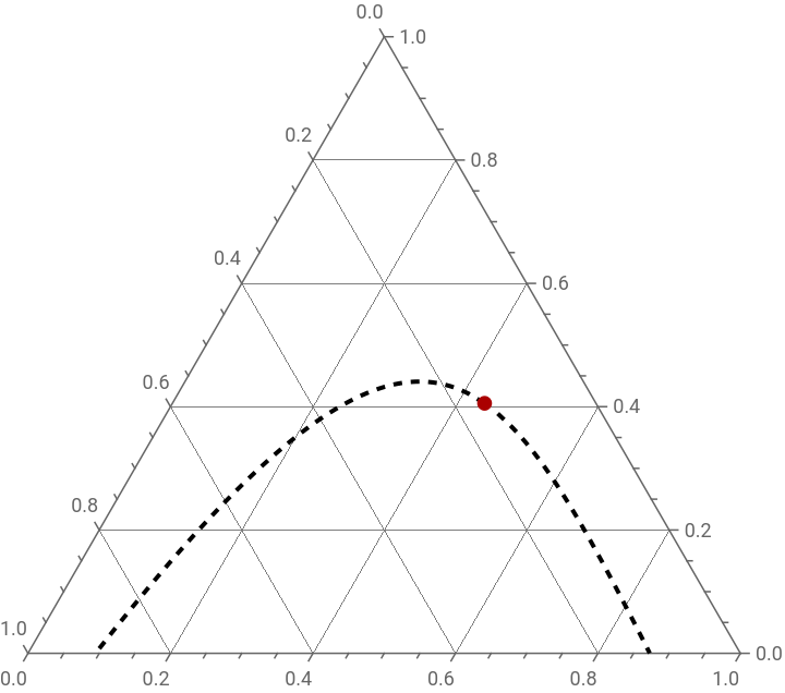
The common tangent method determines the binodal curve by locating pairs of equilibrium compositions that satisfy the equality of tangent planes to the Gibbs free energy of mixing surface. By progressively varying the distance parameter (d), the complete coexistence curve was traced from the plait point to the limits of the two-phase region.
The arc-length continuation method solves the phase-equilibrium equations directly and follows the solution branch continuously using an arc-length constraint. This approach allows robust tracking of the binodal curve, including regions close to the plait point where conventional methods may encounter convergence difficulties.
The resulting ternary phase diagrams obtained from both methods exhibit excellent agreement over the entire two-phase region. The coincidence of the binodal curves confirms the consistency of the NRTL model implementation and demonstrates the reliability of both numerical techniques for predicting ternary LLE behavior. Furthermore, the plait point predicted by the common tangent approach coincides closely with that obtained from arc-length continuation, providing additional validation of the calculated equilibrium data.
Overall, the comparison shows that both methods accurately reproduce the Type-I liquid–liquid equilibrium behavior of the system, with only negligible numerical differences between the predicted coexistence curves.
Method based on common tangent plane
ClearAll["Global`*"];
Universal gas constant
R=1.9872041;
Temperature
T=273.15+45;
NRTL Parameters
param={a13->0.3,a12->0.20,a32->0.30,B12->857.3718000,B21->2650.684300,B13->1410.932300,B31->2291.817900,B23->190.1605000,B32->-153.9573000,A12->-1.969300000,A13->-2.802700000,A23->0.0,A21->-7.132100000,A31->-5.248600000,A32->0.0};
t13=A13+B13/T;t23=A23+B23/T;t12=A12+B12/T;t32=A32+B32/T;t31=A31+B31/T;t21=A21+B21/T;α={{0.,a12,a13},{a12,0.,a32},{a13,a32,0.}}/.param;τ={{0.,t12,t13},{t21,0.,t23},{t31,t32,0.}}/.param;
In[]:=
α//MatrixForm
Out[]//MatrixForm=
0. | 0.2 | 0.3 |
0.2 | 0. | 0.3 |
0.3 | 0.3 | 0. |
In[]:=
τ//MatrixForm
Out[]//MatrixForm=
0. | 0.725567 | 1.6321 |
1.19946 | 0. | 0.597707 |
1.95498 | -0.483914 | 0. |
G[i_,j_]:=Exp[-α[[i,j]]τ[[i,j]]];
COMPOSITION VECTOR
xvec[x1_,x2_]:={x1,x2,1-x1-x2};
NRTL ACTIVITY COEFFICIENTS
lnGamma[i_,x1_,x2_]:=Module[{x,term1,term2},x=xvec[x1,x2];term1=Sum[x[[j]]τ[[j,i]]G[j,i],{j,1,3}]/Sum[x[[k]]G[k,i],{k,1,3}];term2=Sum[x[[j]]G[i,j]/Sum[x[[k]]G[k,j],{k,1,3}](τ[[i,j]]-Sum[x[[m]]τ[[m,j]]G[m,j],{m,1,3}]/Sum[x[[m]]G[m,j],{m,1,3}]),{j,1,3}];term1+term2];gamma[i_,x1_,x2_]:=Exp[lnGamma[i,x1,x2]];
DIMENSIONLESS GIBBS ENERGY OF MIXING: g/RT
gmix[x1_,x2_]:=Module[{x},x=xvec[x1,x2];Sum[x[[i]]Log[x[[i]]],{i,1,3}]+Sum[x[[i]]lnGamma[i,x1,x2],{i,1,3}]];
DERIVATIVES
dgdx1[x1_,x2_]:=Evaluate[D[gmix[u,v],u]/.{u->x1,v->x2}];dgdx2[x1_,x2_]:=Evaluate[D[gmix[u,v],v]/.{u->x1,v->x2}];
UNKNOWNS
vars={x1a,x2a,x1b,x2b,m1,m2};
COMMON TANGENT EQUATIONS
eq1=dgdx1[x1a,x2a]==m1;eq2=dgdx1[x1b,x2b]==m1;eq3=dgdx2[x1a,x2a]==m2;eq4=dgdx2[x1b,x2b]==m2;eq5=gmix[x1b,x2b]-gmix[x1a,x2a]==m1(x1b-x1a)+m2(x2b-x2a);
EXTRA CONSTRAINT - Prevent trivial solution xα=xβ
eq6=(x1b-x1a)^2+(x2b-x2a)^2==d;
first range for d values --- very small d=0.001 yield approximately the plait point
d0t=Table[i,{i,0.001,0.25,0.01}];
Solution
solct=Table[FindRoot[{eq1,eq2,eq3,eq4,eq5,eq6/.d->d0t[[i]]},{{x1a,0.1},{x2a,0.20},{x1b,0.70},{x2b,0.2},{m1,0.45},{m2,0.5}},MaxIterations->1000],{i,1,Length@d0t}];
Second range for d values
d0t=Table[i,{i,0.25,0.60,0.01}];
Solution
solct1=Table[FindRoot[{eq1,eq2,eq3,eq4,eq5,eq6/.d->d0t[[i]]},{{x1a,0.23},{x2a,0.39},{x1b,0.70},{x2b,0.2},{m1,0.55},{m2,-0.15}},MaxIterations->1000],{i,1,Length@d0t}];
Third range for d values
d0t=Table[i,{i,0.6,0.605,0.001}];
Solution
solct3=Table[FindRoot[{eq1,eq2,eq3,eq4,eq5,eq6/.d->d0t[[i]]},{{x1a,0.096},{x2a,0.00076},{x1b,0.871},{x2b,0.00223},{m1,-0.014},{m2,-4.85}},MaxIterations->1000],{i,1,Length@d0t}];
In[]:=
solctf=Join[solct,solct1,solct3];
In[]:=
DATA1ct=Table[{x1a,x2a,1-x1a-x2a}/.solctf[[i]],{i,1,Length@solctf}];DATA2ct=Table[{x1b,x2b,1-x1b-x2b}/.solctf[[i]],{i,1,Length@solctf}];
Pt={{2,1},{0,Sqrt[3.]}}/2;
Type I liquid - liquid equilibrium (LLE) diagram - Plait point indicated in red
p1=ShowTernaryListPlot{DATA1ct,DATA2ct},,Graphics[{Darker@Red,PointSize[0.02],Point[Pt.{DATA1ct[[1]][[1]],DATA1ct[[1]][[2]]}]}]
Out[]=
Method based on arc - length
In[]:=
R=1.987;
Temperature in Kelvin
In[]:=
TK=273.15+45;
NRTL model
In[]:=
GAMMA1=Exp[(t21G21x2+t31G31x3)/(x1+G21x2+G31x3)+x1/(x1+G21x2+G31x3)(-(x2t21G21+x3t31G31)/(x1+G21x2+G31x3))+x2G12/(G12x1+x2+G32x3)(t12-(x1t12G12+x3t32G32)/(G12x1+x2+G32x3))+x3G13/(G13x1+G23x2+x3)(t13-(x1t13G13+x2t23G23)/(G13x1+G23x2+x3))]/.x31-x1-x2;GAMMA1p=Exp[(t21G21xp2+t31G31xp3)/(xp1+G21xp2+G31xp3)+xp1/(xp1+G21xp2+G31xp3)(-(xp2t21G21+xp3t31G31)/(xp1+G21xp2+G31xp3))+xp2G12/(G12xp1+xp2+G32xp3)(t12-(xp1t12G12+xp3t32G32)/(G12xp1+xp2+G32xp3))+xp3G13/(G13xp1+G23xp2+xp3)(t13-(xp1t13G13+xp2t23G23)/(G13xp1+G23xp2+xp3))]/.xp31-xp1-xp2;GAMMA2=Exp[(t12G12x1+t32G32x3)/(G12x1+x2+G32x3)+x1G21/(x1+G21x2+G31x3)(t21-(x2t21G21+x3t31G31)/(x1+G21x2+G31x3))+x2/(G12x1+x2+G32x3)(-(x1t12G12+x3t32G32)/(G12x1+x2+G32x3))+x3G23/(G13x1+G23x2+x3)(t23-(x1t13G13+x2t23G23)/(G13x1+G23x2+x3))]/.x31-x1-x2;GAMMA2p=Exp[(t12G12xp1+t32G32xp3)/(G12xp1+xp2+G32xp3)+xp1G21/(xp1+G21xp2+G31xp3)(t21-(xp2t21G21+xp3t31G31)/(xp1+G21xp2+G31xp3))+xp2/(G12xp1+xp2+G32xp3)(-(xp1t12G12+xp3t32G32)/(G12xp1+xp2+G32xp3))+xp3G23/(G13xp1+G23xp2+xp3)(t23-(xp1t13G13+xp2t23G23)/(G13xp1+G23xp2+xp3))]/.xp31-xp1-xp2;GAMMA3=Exp[(t13G13x1+t23G23x2)/(G13x1+G23x2+x3)+x1G31/(x1+G21x2+G31x3)(t31-(x2t21G21+x3t31G31)/(x1+G21x2+G31x3))+x2G32/(G12x1+x2+G32x3)(t32-(x1t12G12+x3t32G32)/(G12x1+x2+G32x3))+x3/(G13x1+G23x2+x3)(-(x1t13G13+x2t23G23)/(G13x1+G23x2+x3))]/.x31-x1-x2;GAMMA3p=Exp[(t13G13xp1+t23G23xp2)/(G13xp1+G23xp2+xp3)+xp1G31/(xp1+G21xp2+G31xp3)(t31-(xp2t21G21+xp3t31G31)/(xp1+G21xp2+G31xp3))+xp2G32/(G12xp1+xp2+G32xp3)(t32-(xp1t12G12+xp3t32G32)/(G12xp1+xp2+G32xp3))+xp3/(G13xp1+G23xp2+xp3)(-(xp1t13G13+xp2t23G23)/(G13xp1+G23xp2+xp3))]/.xp31-xp1-xp2;G12=Exp[-a12t12];G21=Exp[-a12t21];G13=Exp[-a13t13];G31=Exp[-a13t31];G32=Exp[-a32t32];G23=Exp[-a32t23];t13=A13+B13/TK;t23=A23+B23/TK;t12=A12+B12/TK;t32=A32+B32/TK;t31=A31+B31/TK;t21=A21+B21/TK;
NRTL parameters obtained from Aspen-Plus
In[]:=
param={a130.3,a120.20,a320.30,B12857.3718000,B212650.684300,B131410.932300,B312291.817900,B23190.1605000,B32-153.9573000,A12-1.969300000,A13-2.802700000,A230.0,A21-7.132100000,A31-5.248600000,A320.0};
In[]:=
X1i=0.5;X2i=0.1;sol=FindRoot[{GAMMA1x1GAMMA1pxp1,GAMMA2x2GAMMA2pxp2,GAMMA3(1-x1-x2)GAMMA3p(1-xp1-xp2),L+Lp1,x1L+xp1LpX1i,x2L+xp2LpX2i}/.param,{x2,0.193},{x1,0.058},{xp1,0.900},{xp2,0.035},{L,0.3},{Lp,0.8},AccuracyGoal10,MaxIterations5000];X1=0.5;
Arc-length continuation method
In[]:=
Eq1=GAMMA1x1GAMMA1pxp1/.x1x1[s]/.x2x2[s]/.xp1xp1[s]/.xp2xp2[s]/.LL[s]/.LpLp[s]/.X2X2[s]/.param;Eq2=GAMMA2x2GAMMA2pxp2/.x1x1[s]/.x2x2[s]/.xp1xp1[s]/.xp2xp2[s]/.LL[s]/.LpLp[s]/.X2X2[s]/.param;Eq3=GAMMA3(1-x1-x2)GAMMA3p(1-xp1-xp2)/.x1x1[s]/.x2x2[s]/.xp1xp1[s]/.xp2xp2[s]/.LL[s]/.LpLp[s]/.X2X2[s]/.param;Eq4=L+Lp1/.x1x1[s]/.x2x2[s]/.xp1xp1[s]/.xp2xp2[s]/.LL[s]/.LpLp[s]/.X2X2[s];Eq5=x1L+xp1LpX1/.x1x1[s]/.x2x2[s]/.xp1xp1[s]/.xp2xp2[s]/.LL[s]/.LpLp[s]/.X2X2[s];Eq6=x2L+xp2LpX2/.x1x1[s]/.x2x2[s]/.xp1xp1[s]/.xp2xp2[s]/.LL[s]/.LpLp[s]/.X2X2[s];Eq7=X2'[s]^2+x1'[s]^2+xp1'[s]^2+x2'[s]^2+xp2'[s]^2+L'[s]^2+Lp'[s]^21;
Auxiliary equation
Full DAE system of equations + initial conditions to be solved by NDSolve
Type I liquid-liquid equilibrium (LLE) diagram - Plait point indicated in red
Comparison between both methods shows excellent agreement
CITE THIS NOTEBOOK
CITE THIS NOTEBOOK
Ternary liquid liquid equilibrium using common tangent plane
by Housam Binous
Wolfram Community, STAFF PICKS, June 7, 2026
https://community.wolfram.com/groups/-/m/t/3728851
by Housam Binous
Wolfram Community, STAFF PICKS, June 7, 2026
https://community.wolfram.com/groups/-/m/t/3728851