The Collatz conjecture, or 3x+1 problem, is an unsolved mathematics problem infamous for its ease of explanation yet remarkable difficulty in solvability. The Collatz function relies on choosing a positive integer and continuously repeating the following operations: If the number is even, divide it by two; if the number is odd, multiply it by three and add one. The conjecture states that every positive integer will always reach one. This project uses the Wolfram Language to explore established and potentially new methods of visualizing generalized Collatz functions given by a defined U-function. The numerous phenomena observed include structured distributions of prime number counts in iteration graphs, patterns in digit plots of different bases, and manipulated trajectories using truncated p-adic integers. The observations in the project will hopefully allow others to launch further investigations. This project attempts to visualize the implications of generalized Collatz functions in number theory and geometry from an experimental perspective. An introduction to some representations of generalized Collatz functions precedes the explorations relevant to the aforementioned fields. The treatments described in this project can apply to other generalized Collatz functions. More rigorous analysis is required to appreciate the observations made.
(A word of caution: There are many graphics in this project that need some time to load all the way. Also, the notebook may need to be downloaded for the animations to run smoothly.)
(A word of caution: There are many graphics in this project that need some time to load all the way. Also, the notebook may need to be downloaded for the animations to run smoothly.)
1: Generalizing the Collatz Function
1: Generalizing the Collatz Function
1.1: Introduction to the Collatz Function
1.1: Introduction to the Collatz Function
The Collatz function can be defined as
C(x)
In[]:=
cFunction[x_]:=If[Mod[x,2]==0,x/2,3x+1]
It can be proved that any odd integer that is multiplied by 3 and then added to 1 is even: For with an integer, , which is divisible by 2 and is therefore even. Thus, one arrives at the modified Collatz function , defined as
x2k+1
k
3x+13(2k+1)+12(3k+2)
T(x)
In[]:=
tFunction[x_]:=If[Mod[x,2]==0,x/2,(3x+1)/2]
Given an initial value, one can view the iterations of and its cycle.
C(x)
In[]:=
NestList[cFunction,11,20]
Out[]=
{11,34,17,52,26,13,40,20,10,5,16,8,4,2,1,4,2,1,4,2,1}
By definition, follows a similar trajectory but in less iterations. It also has one less element in its cycle.
T(x)
In[]:=
NestList[tFunction,11,20]
Out[]=
{11,17,26,13,20,10,5,8,4,2,1,2,1,2,1,2,1,2,1,2,1}
Focusing on , one can view these iterations in multiple ways including graphs and binary integer length trajectory plots.
T(x)
Graph of the sequence:
T(11)
Out[]=

Trajectory of over 20 iterations:
T(11)
Out[]=
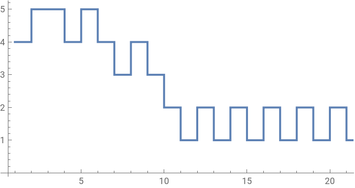
If the Collatz conjecture is true, then every positive integer inputted to should reach the same cycle of
T(x)
In[]:=
FindCycle[NestGraph[tFunction,11,20]]
Out[]=
{{21,12}}
It is apparent through a plot of the first 50 numbers that some initial values take longer than others to fall into cycle.
Series of trajectories of the first 50 numbers inputted to over 75 iterations:
T(x)
Out[]=
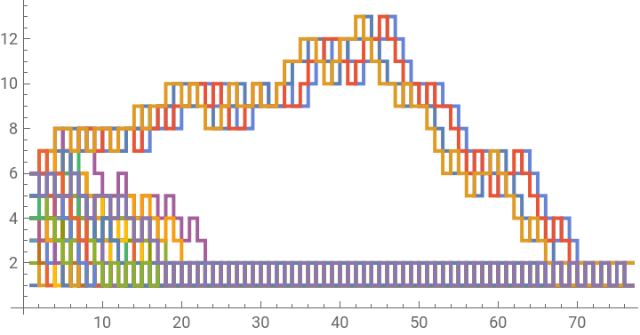
Each successive iteration of can be viewed. For the 1st iteration of the first 50 numbers:
T(x)
In[]:=
#->tFunction[#]&/@Range[50]
Out[]=
{12,21,35,42,58,63,711,84,914,105,1117,126,1320,147,1523,168,1726,189,1929,2010,2132,2211,2335,2412,2538,2613,2741,2814,2944,3015,3147,3216,3350,3417,3553,3618,3756,3819,3959,4020,4162,4221,4365,4422,4568,4623,4771,4824,4974,5025}
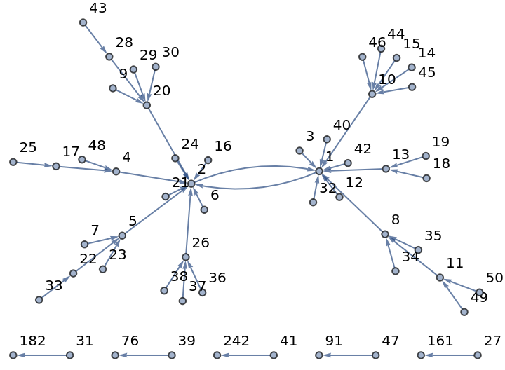
At the 7th iteration, one can see how many numbers have reached the cycle and how many have not.
In[]:=
#->Nest[tFunction,#,7]&/@Range[50]
Out[]=
{12,21,31,42,52,62,75,81,920,101,118,121,131,1410,1510,162,174,1813,1913,202,212,225,235,242,2517,262,27161,2820,2920,3020,31182,321,3322,348,358,3626,3726,3826,3976,401,41242,421,4328,4410,4510,4610,4791,484,4911,5011}
Graph of the 7th iteration of the first 50 numbers inputted to :
T(x)
Out[]=
It is possible to have a negative integer as an initial value. In that case, there are 3 possible cycles for a number to fall into.
In[]:=
NestList[tFunction,-1,1]
Out[]=
{-1,-1}
In[]:=
NestList[tFunction,-5,3]
Out[]=
{-5,-7,-10,-5}
In[]:=
NestList[tFunction,-17,11]
Out[]=
{-17,-25,-37,-55,-82,-41,-61,-91,-136,-68,-34,-17}
1.2: Expressing the Collatz Function as a Single Function
1.2: Expressing the Collatz Function as a Single Function
Since the conditional for is based on the parity of the input, then one can arrive at the function where is 0 if is even and 1 if is odd. The switch-Collatz function can be defined by
T(x)
T(x,s)+x+s
(1-s)x+s(3x+1)
2
x
2
1
2
s
x
x
S(x)
In[]:=
sFunction[x_]:=x/2+(x+1/2)Mod[x,2]
Instead of a modulo operator for , a sine function can be used: Define (x) as
s
S
sin
In[]:=
sFunctionSin[x_]:=x/2+(x+1/2)Sin[xPi/2]^2
By the Pythagorean identity, define (x) as
S
cos
In[]:=
sFunctionCos[x_]:=(3x+1)/2-(x+1/2)Cos[xPi/2]^2
T(x)
S(x)
S
sin
S
cos
In[]:=
NestList[sFunctionCos,11,10]==NestList[sFunctionSin,11,10]==NestList[sFunction,11,10]==NestList[tFunction,11,10]
Out[]=
True
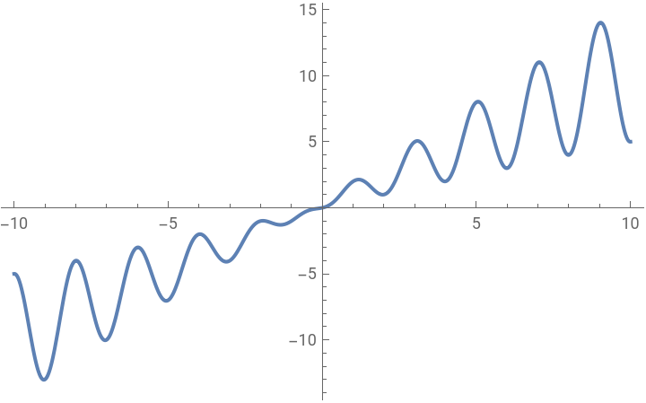
Including a sine or cosine function implies the initial value is no longer restricted to the integers, instead expanding the domain to the reals.
Plot of (x) over :
S
sin
[-10,10]
Out[]=
1.3: Expressing the Collatz Function with FRACTRAN
1.3: Expressing the Collatz Function with FRACTRAN
1.4: Generalizing the Collatz Function with the U-function
1.4: Generalizing the Collatz Function with the U-function
2: Iteration Behavior
2: Iteration Behavior
2.1: Search Methods
2.1: Search Methods
The search methods for determining systems/initial values with interesting behavior are as follows: The single plot search is the standard method, but hard to compare with other systems/initial values at the same time.
One can perform an expanded and narrow initial value search by multiplying the initial value and then adding to it.
One can perform an expanded and broad initial value search by adding to the initial value and then multiplying it.
2.2: Trajectories
2.2: Trajectories
It is apparent that some trajectories converge to others after a certain number of iterations.
In fact, “shifted” trajectories are also apparent.
To quantify the behavior of these systems, it is necessary to implement a sort of classifier. One can find the mean of each trajectory over every iteration for a sample of initial values.
It is possible to determine the mean of every trajectory at each iteration for a sample of initial values instead.
One can define a metric of balance as the rate of change between the mean of the initial inputs and the mean of the mean of every trajectory in the sample at each iteration. The rate of change indicates a system is more balanced if it is closer to 0, with its sign indicating the direction of the system, i.e. negative implying the system is heading towards a cycle and positive indicating the system is diverging. The number of iterations can be extended to determine if the system becomes more or less balanced.
2.3: Cycles
2.3: Cycles
So-called “monster” cycles can also be observed.
To begin classifying cycle behavior, one can implement a cycle counter which can be applied to a desired iteration.
One can also determine the maximum cycle length at a given iteration.
One can generate cycle information of a system up to a desired iteration; specifically, the number of iterations until a cycle (if it exists) and the length of that cycle.
One can use this cycle information to show the initial values that have reached a cycle after a certain number of iterations, or their halting time, and those that have not, which is indicated by a lip at the bottom of the following plot.
The cycle information can instead show which initial values are not in cycle after a certain number of iterations. (In the plot below, a value of 1 indicates the initial value is not in a cycle while a value of 0 indicates the initial value is in a cycle.)
3: Prime Number Distributions
3: Prime Number Distributions
3.1: Prime Count Distributions
3.1: Prime Count Distributions
Prime numbers are always a relevant topic in mathematics. It is possible to plot the distribution of primes in different bases.
Plotted normally in base 10, the distribution of the primes is not too revealing. (In the plot below, the color red indicates a prime number and the color black indicates a composite number.)
Distribution of primes up to 100 in base 10:
However, structures begin to appear for certain bases.
3.2: Twin Prime Count Distributions
3.2: Twin Prime Count Distributions
The distribution of twin primes is also consistent for the first few iterations. (For the following plots, the color white indicates systems with the least count of twin primes, which progresses to the color black, or the system with the greatest count of twin primes.)
The distributions of the pairs of twin primes contains the most structure. (For the following plots, the color white indicates systems with the least count of twin prime pairs, which progresses to the color black, or the system with the greatest count of twin prime pairs.)
The twin prime tower disappears when the iteration is increased.
Another feature that can be identified for larger initial values is a twin prime “staircase” which behaves like a twin prime tower, only along a diagonal.
By removing any repeating values in a system, a twin prime staircase can be represented as a twin prime “shelf” to show the continuation of the twin prime pair. (In the plot below, the color orange indicates the number is a twin prime and the color black the number is not a twin prime.)
4: Repeating Structures
4: Repeating Structures
4.1 Patterned Structures
4.1 Patterned Structures
It is hard to identify any patterns in such a large base, so consider converting the numbers in the sequence to binary and then reversing the digits. (In the plot below, the color pink indicates 0 and the color black indicates 1.)
The structure is made of a series of triangles, forming what looks like a sort of mountain range. In base 3, the structure is still constituted of triangles, this time oriented in the opposite direction.
It is easy to understand that the most pink triangles, or 0-triangles, occur when the initial value is a power of 2. To obtain a triangle that is mostly black, or a 1-triangle, the initial condition must be a binary string of 1’s, equivalently the difference between a power of 2 and 1 in decimal.
A 1-triangle appears in the bottom right corner as expected. Multiplying the previous initial value by a power of 2 shifts this black region and forms a pink triangle as well. The black region appears to have precedence over the pink region.
The structure can be manipulated further with a logical progression of the previous initial value.
The structure is consistent until the digits are converted to base 3, where it appears to fall apart.
Knowing a 1-triangle is the result of an initial value being a binary string of 1’s, one can interject a 0 somewhere in this string of 1’s to create self-contained structures. Self-contained “inverse” cycles as also apparent until the length of the 1-triangle.
Again converting the digits to base 3, the 1-triangle reverses its orientation and the inverse cycle is still present.
4.2: Something Alive
4.2: Something Alive
By partitioning the digits of such structures in different groups, one can notice “wavy” behavior for certain systems/initial values.
4.3: Trajectories with Special Initial Values
4.3: Trajectories with Special Initial Values
Knowing the behavior of the digit plot structures, one can begin to manipulate the trajectories of certain systems. Consider an initial value of a truncated 10-adic integer, such as 2:
The trajectories of such initial values appear to almost always have the same slope.
The consecutive negative trajectory slope for the a certain number of iterations is explained by the increasing powers of 2 in the prime factorization of the initial values.
An input that previously led to a 1-triangle, or the difference between 2 to an increasing power and 1, results in a consecutive positive trajectory slope for as many iterations as the value of the power chosen.
5: Concluding remarks
5: Concluding remarks
5.1: The Future
5.1: The Future
5.2: Extra Stuff
5.2: Extra Stuff
Complex rule 1 with an initial value of 1:
Complex rule 2 with an initial value of 1:
Complex rule 3 with an initial value of 1:
Complex rule 4 with an initial value of 1:
Complex rule 5 with an initial value of 1:
Keywords
Keywords
◼
Generalized Collatz function
◼
Iteration
◼
Trajectory
◼
Cycle
◼
Prime number
◼
Digit plot
Acknowledgment
Acknowledgment
Special thanks to Stephen Wolfram for suggesting this project, as well as to my mentor Brad Klee and the rest of the NKS members - Ben Peter, Bowen Ping, Johannes Martin, and Zsombor Meder - for their feedback and support throughout the project. Thanks to everyone at WSS 2023 who made it such a great time!
References
References
CITE THIS NOTEBOOK
CITE THIS NOTEBOOK
Exploring generalized Collatz functions
by Russell Martinez
Wolfram Community, STAFF PICKS, July 12, 2023
https://community.wolfram.com/groups/-/m/t/2959684
by Russell Martinez
Wolfram Community, STAFF PICKS, July 12, 2023
https://community.wolfram.com/groups/-/m/t/2959684