Additive continuous cellular automata (ACCAs) extend traditional cellular automata by allowing real-valued states and additive update rules. Like differential equations, they can exhibit stable or unstable behavior depending on how small perturbations evolve. This project investigates the stability of ACCAs by introducing localized perturbations and analyzing their divergence over time. We focus on the formation and geometry of error fronts—boundaries separating regions of convergence and divergence—and explore how different rule weights influence their propagation.
Introduction
Introduction
Stability
Stability
Stability describes how a dynamical system evolves in response to small disturbances in its initial conditions. A system is said to be in a steady state or in equilibrium when its variables remain constant (or follow a fixed pattern) over time. Stability analysis asks whether a system will converge to such a state after small perturbations to initial conditions, or if it will diverge as time progresses.
In the study of differential equations, many systems cannot be solved analytically, or be efficiently approximated numerically. As a result, we often use qualitative methods to understand their behavior near equilibrium points. One such method is linearization, where the system is approximated near an equilibrium by its Jacobian matrix; the signs of the eigenvalues then indicate local stability. A more general method involves constructing Lyapunov functions which are scalar functions that can allow us to assess stability over larger regions and even globally [1].
These tools allow us to understand the evolution of complex systems without requiring exact solutions. However, for continuous cellular automata, such a theory of stability is still underdeveloped. By studying how perturbations spread or decay in additive continuous cellular automata, we aim to develop a parallel understanding of stability for these discrete-time systems.
Continuous Cellular Automata
Continuous Cellular Automata
Cellular automata are discrete models that study how local rules can give rise to complex global dynamics. The simplest form of these models is the one-dimensional elementary cellular automata, where each cell on a one-dimensional grid holds a binary state ( or ), and updates its state based on the values of its neighbors, according to a fixed rule. These updates occur in discrete time steps and are visualized row by row, often revealing intricate and surprising patterns. Rules for the one-dimensional elementary cellular automata are often described by a Boolean function of neighboring cells :
0
1
f:{0,1}
3
{0,1}
(n+1)
x
i
(n)
x
i-1
(n)
x
i
(n)
x
i+1
where ∈{0,1} represents the state of cell at time .
(n)
x
i
i
n
Continuous cellular automata generalize the elementary cellular automata by allowing cells to hold real-valued states. In this notebook, we focus on two representative examples, additive continuous cellular automata, and coupled map lattices.
Additive Continuous Cellular Automata
Additive Continuous Cellular Automata
Additive continuous cellular automata (ACCA) extend the one-dimensional elementary cellular automata framework by allowing cells to evolve through linear combinations of neighboring cells. Rules for the one-dimensional ACCA are real-valued functions :
f:R
3
R
(n+1)
x
i
(n)
x
i-1
(n)
x
i
(n)
x
i+1
(n)
x
i-1
(n)
x
i
(n)
x
i+1
for real constants , , and . To restrict the range of this function to the interval , we can either apply a iterated map (such as the logistic map or the tent map) on the output of , or reduce modulo 1:
a
b
c
[0,1]
f
f
(n+1)
x
i
(n)
x
i-1
(n)
x
i
(n)
x
i+1
(n+1)
x
i
(n)
x
i-1
(n)
x
i
(n)
x
i+1
Both approaches enable richer dynamics and generate intriguing visualizations. Please see Function & Variable Definitions for graphs of these functions.
Coupled Map Lattice
Coupled Map Lattice
Coupled map lattices (CML) are another type of continuous cellular automaton in which a nonlinear map is applied to each cell before spatial interactions (addition). The output of the map is then averaged with the outputs of neighboring cells, scaled by a coupling strength parameter . The standard rule for the one-dimensional CML is a function :
ϵ∈[0,1]
f:[0,1]
3
[0,1]
(n+1)
x
i
(n)
x
i-1
(n)
x
i
(n)
x
i+1
(n)
x
i
ϵ
2
(n)
x
i-1
(n)
x
i+1
This introduces both nonlinear dynamics and spatial interaction, making CMLs especially useful for studying spatiotemporal chaos and pattern formation.
Linking to Differential Equations
Linking to Differential Equations
Additive continuous cellular automata and coupled map lattices are discrete-time systems that share important similarities with differential equations. The table below highlights how different models vary in whether they treat space, time, and state as discrete (D) or continuous (C) [2]:
Out[]=
Model | Space | Time | State |
Elementary Cellular Automata | D | D | D |
Continuous Cellular Automata | D | D | C |
Coupled Ordinary Differential Equation | D | C | C |
Partial Differential Equation | C | C | C |
These connections motivate the use of tools like stability analysis and perturbation methods to better understand the behavior of continuous cellular systems.
Perturbation Dynamics in Continuous Cellular Automata
Perturbation Dynamics in Continuous Cellular Automata
To understand the stability of continuous cellular automata, we investigate how small changes in the initial state of a single cell evolve over time. This approach is inspired by techniques used in ordinary differential equations, where small perturbations are introduced to systems to observe whether they grow, decay, or remain bounded. In the context of CCAs, we can track how localized disturbances propagate through time by comparing the perturbed evolution against an unperturbed baseline.
Models & Observations
Models & Observations
Visualizations of Continuous Cellular Automata
Visualizations of Continuous Cellular Automata
This exploration begins with the implementation of the rules described above:
In[]:=
ACCARuleMap[list_?ListQ,a_?NumericQ,b_?NumericQ,c_?NumericQ,map_]:=map[aRotateLeft[list]+blist+cRotateRight[list]];ACCARuleMod[list_?ListQ,a_?NumericQ,b_?NumericQ,c_?NumericQ]:=Mod[aRotateLeft[list]+blist+cRotateRight[list],1];CMLRule[list_?ListQ,ϵ_?NumericQ,map_]/;0<=ϵ<=1:=(1-ϵ)map[list]+(map[RotateLeft[list]]+map[RotateRight[list]]);
ϵ
2
These rules will be applied iteratively using the function, where the initial state will consist of a single active (nonzero) cell. In this discussion, this cell will be centered on a grid of 201 cells and given a value of .
NestList
Pi/6
In[]:=
initialState=CenterArray[N[Pi/6,100],201];
States of the cellular automaton can be visualized on a grid by assigning a color to all values between 0 and 1. The color function used in these images is shown below:
In[]:=
BarLegend[{"DeepSeaColors",{0,1}},LegendLayout->"Row",LegendMarkerSize->{400,30}]
Out[]=

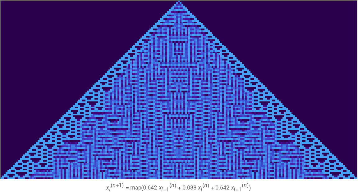
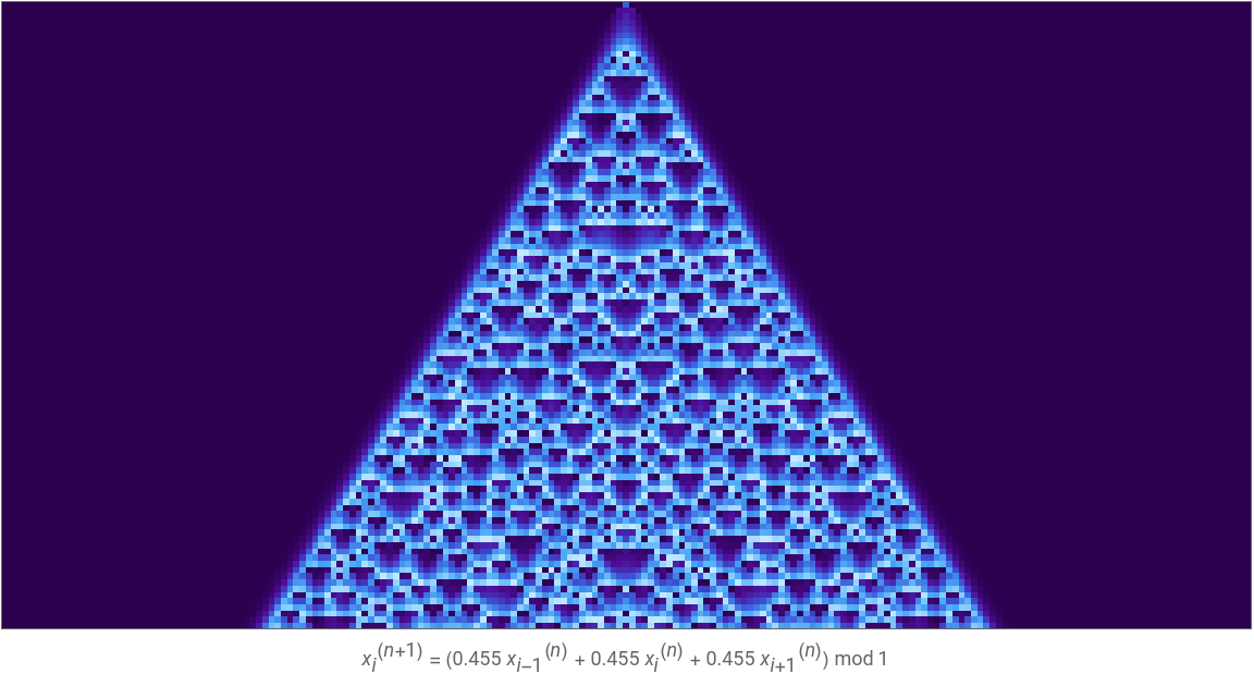
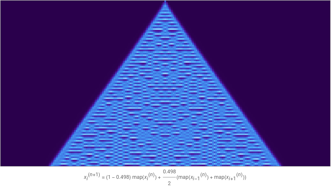
Some interactive graphics of the rules discussed above are provided below:
Out[]=


Out[]=
Out[]=
Selected Visualizations
Selected Visualizations
Analyzing Stability
Analyzing Stability
To assess the stability of these systems, we can introduce small perturbations to the active cell in the first state:
By increasing the size of these perturbations, we can visually perceive the movement of an error front, which is the boundary beyond which the perturbed system begins to diverge significantly from the unperturbed reference. While this front imperceptible in static visualizations, it becomes immediately apparent when the perturbation is varied over time.
This effect is related to second-order short-range motion, a phenomenon in visual neuroscience where motion is inferred not from luminance-defined features (first-order motion), but rather from changes in higher-order properties such as contrast, texture, or spatial correlations. In our case, the evolving structural difference between the perturbed and unperturbed systems allows us to track the spread of the disturbance [3].
In each of these examples, an error front emerges as the magnitude of perturbation is increased.
Identifying the Error Front
Identifying the Error Front
To identify the error front between a perturbed and unperturbed evolution of a continuous cellular automaton, we will compute the element-wise absolute difference between the two data arrays at each time step. This gives us a temporal sequence of difference profiles.
To visualize the divergence front, we create a Boolean mask that marks all cells after the divergence time in each column, making the transition clearly visible. By masking the unperturbed region before divergence and the perturbed region after, we can combine both plots to isolate the difference. Below is an image of the ACCA using the modulo-1 rule:
We can also animate how this error front propagates through the system over time, for each of the three examples shown in the previous section.
In the ACCA using the logistic map, the error front propagates irregularly across the system, frequently changing shape.
In the ACCA using the modulo-1 function, the error front propagates regularly across the system, forming a relatively smooth curve.
In the CML using the tent map, the error front propagates irregularly across the system, similar to the first example.
Discussions
Discussions
Error Front Geometry
Error Front Geometry
In the example above, perturbations propagate outwards along a symmetric front, which appears hyperbolic in shape. This regularity, however, is not observed across the entire parameter space. Negative weights, nonlinear maps, and certain asymmetrical weights distort the front, often leading to unpredictable outcomes. Modeling the exact curve in these cases remains a challenge. More sophisticated methods should also be considered in cases where errors propagate diagonally, or in regions, to allow for better visualization of regions of divergence.
Localized Divergence
Localized Divergence
The current method for identifying error fronts assumes that once two systems diverge, they remain divergent. However, this may overlook cases where the systems temporarily diverge and later reconverge. These transient deviations are not captured by a single divergence time, potentially underestimating the true extent of instability. A more robust approach would involve tracking divergence over a sliding time window to better account for these intermittent behaviors.
Numerical Precision
Numerical Precision
which requires many digits of precision:
On the contrary, the second row manually specifies precision (up to 100 digits), either after symbolic evaluation, or before (that is, starting with a numeric initial condition). These cases plot successfully.
Irrational Numbers
Irrational Numbers
For example, with the initial condition 1/2, we generate the greyscale Sierpinski triangle:
Coupling with Spatial Masks
Coupling with Spatial Masks
By allowing each cell’s coupling to depend on its corresponding elementary cellular automaton value, we can generate structured zones of periodicity and chaos. Despite using simple rules, the resulting dynamics under the logistic map reveal rich spatiotemporal structure. While not studied in depth, these results merit further exploration.
Concluding Remarks
Concluding Remarks
This project develops continuous cellular automata models to visualize the dynamics of nonlinear update rules. By introducing localized perturbations, we observe the emergence of hyperbolic error fronts that separate regions of convergence and divergence under the modulo-1 rule, and more irregular fronts in systems governed by iterated maps. Additionally, we demonstrate how binary cellular automata can serve as spatial masks in coupled map lattices, producing structured zones of periodicity and chaos.
Future Works
Future Works
Future work includes analytical characterization of the shape and speed of error fronts under the modulo-1 rule with arbitrary neighbor weights, with generalizations to larger neighborhoods. Further analysis of more complex initial conditions, beyond a single central cell, may offer a richer understanding of stability across the system. This direction may also support the application of Lyapunov stability theory to continuous cellular automata.
Acknowledgments
Acknowledgments
I would like to thank my mentors Pietro, for his guidance in shaping the direction of this project and in helping refine its focus, and Sotiris, for suggesting insightful avenues to explore and sharing valuable resources. I am also grateful to Karina Ho and the entire Wolfram Summer School cohort of mentors and students for their support and encouragement during the program.
References
References
1
.R. Murray, S. Sastry, and L. Zexiang, “A Mathematical Introduction to Robotic Manipulation,” Association for Computing Machinery. https://dl.acm.org/doi/10.5555/561828.
2
.K. Kaneko and T. Yanagita (2014), “Coupled maps,” Scholarpedia. http://dx.doi.org/10.4249/scholarpedia.4085.
3
.G. Mather and P. Cavanagh (1989), “Motion: The long and short of it,” Spatial Vision. https://doi.org/10.1163/156856889X00077.
Cite This Notebook
Cite This Notebook
Stability Analysis of Additive Continuous Cellular Automata
by Tarang Janawalkar
Wolfram Community, July 9, 2025
https://community.wolfram.com/groups/-/m/t/3494918
by Tarang Janawalkar
Wolfram Community, July 9, 2025
https://community.wolfram.com/groups/-/m/t/3494918