Fixing the bugs
Fixing the bugs
There are a few main problems with our previous analysis: ConvexHullRegion was a bad idea, we did not have date-sensitive distance parameters, and the lunar limb was chosen arbitrarily. If we just fix the first two, we can turn our initial failed experiment into a total success. A hint how to do so was given by Ernie Wright of NASA GSFC who pointed us to a talk he gave back in 2017. Let’s now see how calculations turn out if we’re a bit more careful.
The relevant parameters are obtained from system as:
In[]:=
eclipse=SolarEclipse[]rs=Entity["Star","Sun"]["Radius"];rm=Entity["PlanetaryMoon","Moon"]["Radius"];dse=AstroDistance["Sun",{"Earth",eclipse}];dme=AstroDistance["Moon",{"Earth",eclipse}];
Out[]=
To test for sensitivity to the distance ratio, let’s calculate a pair of conic sections and see how they overlap the origin in the fundamental plane:
Out[]=
The green circle is projected from one point on the solar limb, while the blue circle is the “pinhole” projection through the lunar limb. Since the red dot is inside green and outside blue, it looks like an eclipse could possibly happen. The natural parameters are so close to an edge case that if we even mistake them by 10%, then we get circumstances where an eclipse would not happen:
Out[]=
Having noticed that, let’s keep the good parameters, and move on to calculating umbra tangents as seen in Ernie’s talk. Our previous attempt using ConvexHullRegion wasn’t entirely stupid and had one nice feature that it only depended on a point-set output, and not on a choice between the two projection models. Now that we’re going on to an envelope method, we have to choose a projection model, so let’s just compare both.
We start by generating decently high-precision data, one point per degree on the sun and ten points per degree on the moon. Then we calculate a few point sets by downsampling the lunar limb, and produce depictions, first for the more obvious model which projects from one point on the solar limb:
Out[]=
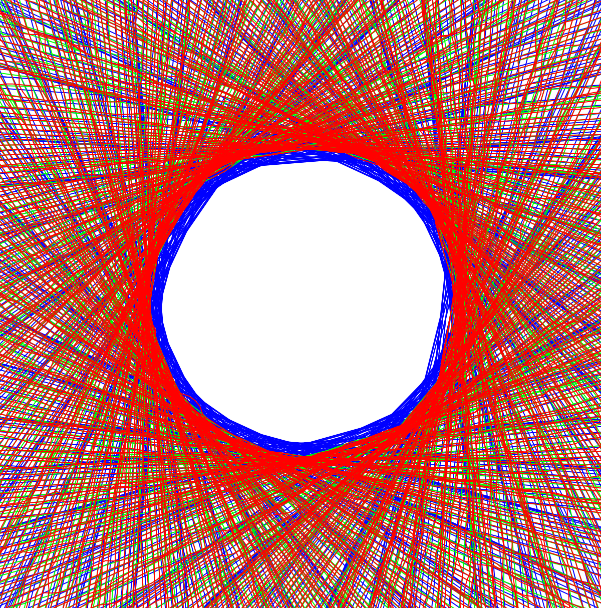
This is a mess, especially because the boundaries are not circular, as is very noticeable with the valley to the southwest. The model projecting through pinholes on the lunar limb produces much clear results, but the layers need to be reversed:
Out[]=
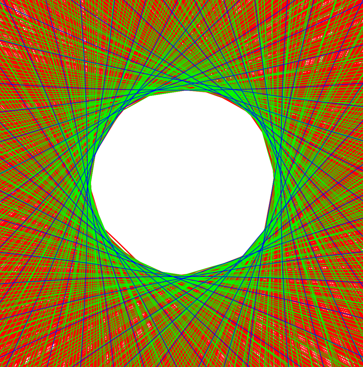
Some edges overlap red blue and green or just red and green, which strongly suggests that the projection procedure will converge given enough sample points. But what is causing that surprise edge to the southwest? Per Jose’s suggestion, we can use Tooltip to find out:
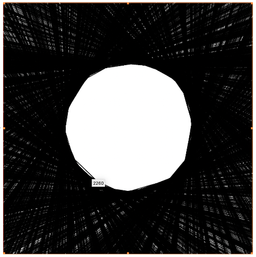
Checking this index against the lunar limb data, we find a deep and narrow valley that could easily be skipped over entirely if the data was thinned out by a factor of 10 or more:
Now that we seem to have the math problem figured out, let’s see if we can make one more image that’s dressed up enough for a magazine cover. In this case, RegionUnion returns a topological annulus, and we can then extract the central hole and plot above the tangents:
Our minimal working example shows that the polygon umbra effect is due to the profile of the lunar limb, and supports the “double diamonds on corners” ideas. This is true especially because edges can be put into correspondence with points on the lunar limb. Now let’s see if observational scientists can see the effect in April. Jeff Bryant says it may be more difficult this year due to apparent sizes of sun and moon being too different.