The liquid–liquid equilibrium (LLE) of the water + n-butanol system was calculated using the NRTL activity-coefficient model with binary interaction parameters obtained from Ref. 1. The coexistence compositions were determined by solving the equality of component activities in the two liquid phases over the temperature range 273.15–353.15 K.
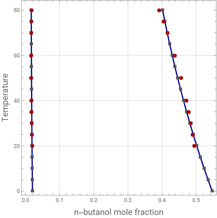
The calculated binodal curve shows good agreement with the experimental data (obtained from Ref. 2). As the temperature increases, the mutual solubility of the two components increases, resulting in a gradual reduction of the miscibility gap. The NRTL model accurately reproduces both the aqueous-phase composition and the butanol-rich phase composition, confirming the suitability of the selected interaction parameters for representing the phase behavior of this partially miscible system.
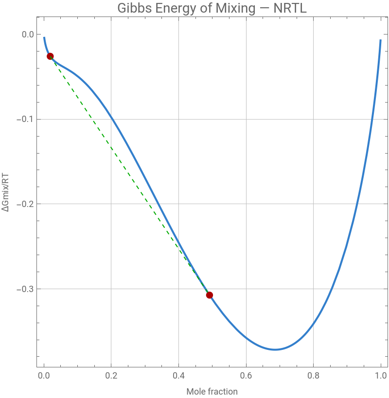
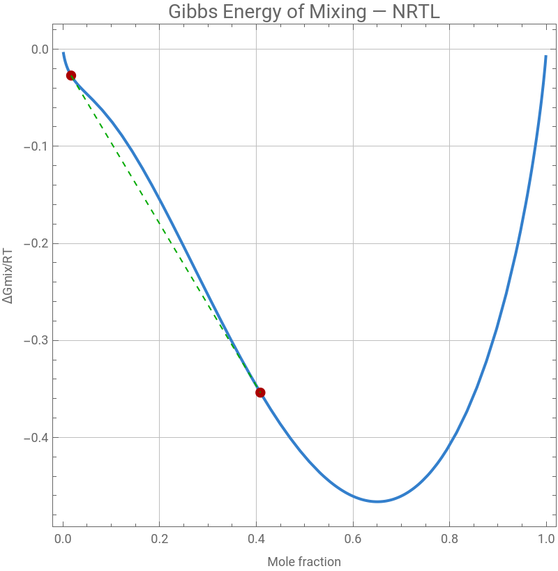
To verify thermodynamic consistency, the dimensionless Gibbs free energy of mixing, ΔGmix/RT, was evaluated at different temperatures. The coexistence compositions obtained from the LLE calculations lie on a common tangent to the Gibbs energy curve. At 298.15 K, the first derivative of ΔGmix/RT at the two equilibrium compositions is identical (−0.59547), while at 348.15 K the corresponding slopes are also equal (−0.83441). This confirms satisfaction of the common-tangent criterion and demonstrates that the calculated phase compositions correspond to thermodynamically stable liquid–liquid equilibrium states.
Overall, the NRTL model provides an accurate description of the liquid–liquid equilibrium and Gibbs energy behavior of the water + n-butanol system over the investigated temperature range.
NRTL model for activity coefficients - temperature-dependent binary interaction parameters and nonrandomness parameters are obtained from Ref. 1
Gam[i_,T_]:=Exp(t[j,i,T]G[j,i,T]x[j])(G[l,i,T]x[l])+(G[l,j,T]x[l])t[i,j,T]-(t[r,j,T]G[r,j,T]x[r])(G[l,j,T]x[l])/.x[1]x1/.x[2]1-x1;Gamp[i_,T_]:=Exp(t[j,i,T]G[j,i,T]x[j])(G[l,i,T]x[l])+(G[l,j,T]x[l])t[i,j,T]-(t[r,j,T]G[r,j,T]x[r])(G[l,j,T]x[l])/.x[1]xp1/.x[2]1-xp1;G[i_,j_,T_]:=Exp[-a[i,j]t[i,j,T]];
2
∑
j=1
2
∑
l=1
2
∑
j=1
G[i,j,T]x[j]
2
∑
l=1
2
∑
r=1
2
∑
l=1
2
∑
j=1
2
∑
l=1
2
∑
j=1
G[i,j,T]x[j]
2
∑
l=1
2
∑
r=1
2
∑
l=1
Data from Ref. 1
t[1,2,T_]:=−3.74+795.6/T;t[2,1,T_]:=8.69-1057.5/T;t[1,1,T_]:=0.0;t[2,2,T_]:=0.0;a[1,2]=0.20;a[2,1]=0.20;
Clear[T,sys];
In[]:=
sys[T_]:={x1*Gam[1,T]==xp1*Gamp[1,T],(1-x1)*Gam[2,T]==(1-xp1)*Gamp[2,T]};
In[]:=
sol[T_]:=FindRoot[sys[T],{{x1,0.0005},{xp1,0.50}},AccuracyGoal->10,PrecisionGoal->8,MaxIterations->500];
In[]:=
mydata=Table[{i,x1/.sol[i],xp1/.sol[i]},{i,273.15,353.15,5}]
Out[]=
{{273.15,0.020333,0.547108},{278.15,0.0199539,0.535117},{283.15,0.0196053,0.523579},{288.15,0.019284,0.512481},{293.15,0.0189871,0.50181},{298.15,0.0187123,0.491553},{303.15,0.0184574,0.481695},{308.15,0.0182206,0.47222},{313.15,0.0180001,0.463114},{318.15,0.0177946,0.454361},{323.15,0.0176028,0.445945},{328.15,0.0174234,0.437853},{333.15,0.0172554,0.430069},{338.15,0.0170979,0.42258},{343.15,0.0169502,0.415372},{348.15,0.0168113,0.408433},{353.15,0.0166807,0.40175}}
In[]:=
p1=ListPlot[{Transpose@{mydata[[All,2]],mydata[[All,1]]-273.15},Transpose@{mydata[[All,3]],mydata[[All,1]]-273.15}},PlotMarkers->{Style["■",12,Darker@Gray],Style["■",12,Darker@Gray]},PlotStyle->Darker@Blue,Joined->True,Frame->True,AspectRatio->1,GridLines->Automatic];
Experimental data from Ref. 2
data2exp={{293.2,0.02,0.4944},{298.2,0.0189,0.4898},{303.2,0.0181,0.4846},{308.2,0.0174,0.4785},{313.2,0.017,0.4718},{323.2,0.0164,0.4562},{333.2,0.0164,0.4377},{343.2,0.0169,0.4164},{348.2,0.0173,0.4045},{353.2,0.0179,0.3916}};
In[]:=
p2=ListPlot[{Transpose@{data2exp[[All,2]],data2exp[[All,1]]-273.15},Transpose@{data2exp[[All,3]],data2exp[[All,1]]-273.15}},PlotMarkers->{Style["●",10,Darker@Red],Style["●",10,Darker@Red]},Frame->True,AspectRatio->1,GridLines->Automatic];
Comparison between our predicted data using NRTL model (gray rectangles) and the experimental data (red dots) reported in Ref: 2
Show[p1,p2,PlotRange->All,FrameLabel->{Style["n-butanol mole fraction",14],Style["Temperature",14]}]
Out[]=
At T = 298.15 K
Gibbs Energy of Mixing—visualise instability region
GmixNRTL=(x1*Log[x1*Gam[1,T]]+x2*Log[x2*Gam[2,T]]/.x2->1-x1/.T->298.15);
In[]:=
plotGmix=Plot[GmixNRTL,{x1,0.001,0.999},PlotStyle->{Thick,RGBColor[0.2,0.5,0.8]},PlotRange->All,PlotLabel->Style["Gibbs Energy of Mixing — NRTL",14],GridLines->Automatic,GridLinesStyle->Lighter[Gray,0.5],Frame->True,FrameLabel->{"Mole fraction","ΔGmix/RT"},ImageSize->400,Frame->True,AspectRatio->1,GridLines->Automatic];
In[]:=
Show[plotGmix,Graphics[{PointSize[0.02],Darker@Red,Point[{x1,GmixNRTL}/.x1->mydata[[6,2]]],Point[{x1,GmixNRTL}/.x1->mydata[[6,3]]],Dashed,Darker@Green,Line[{{x1,GmixNRTL}/.x1->mydata[[6,2]],{x1,GmixNRTL}/.x1->mydata[[6,3]]}]}]]
Out[]=
In[]:=
D[GmixNRTL,x1]/.x1->mydata[[6,2]]
Out[]=
-0.59547
In[]:=
D[GmixNRTL,x1]/.x1->mydata[[6,3]]
Out[]=
-0.59547
At T = 348.15 K
Gibbs Energy of Mixing—visualise instability region
GmixNRTL=(x1*Log[x1*Gam[1,T]]+x2*Log[x2*Gam[2,T]]/.x2->1-x1/.T->348.15);
In[]:=
plotGmix=Plot[GmixNRTL,{x1,0.001,0.999},PlotStyle->{Thick,RGBColor[0.2,0.5,0.8]},PlotRange->All,PlotLabel->Style["Gibbs Energy of Mixing — NRTL",14],GridLines->Automatic,GridLinesStyle->Lighter[Gray,0.5],Frame->True,FrameLabel->{"Mole fraction","ΔGmix/RT"},ImageSize->400,Frame->True,AspectRatio->1,GridLines->Automatic];
In[]:=
Show[plotGmix,Graphics[{PointSize[0.02],Darker@Red,Point[{x1,GmixNRTL}/.x1->mydata[[16,2]]],Point[{x1,GmixNRTL}/.x1->mydata[[16,3]]],Dashed,Darker@Green,Line[{{x1,GmixNRTL}/.x1->mydata[[16,2]],{x1,GmixNRTL}/.x1->mydata[[16,3]]}]}]]
Out[]=
In[]:=
D[GmixNRTL,x1]/.x1->mydata[[16,2]]
Out[]=
-0.834412
In[]:=
D[GmixNRTL,x1]/.x1->mydata[[16,3]]
Out[]=
-0.834412
References
References
[1] Danielle L. de Klerk and Cara E. Schwarz, Simplified Approach to the Parameterization of the NRTL Model for Partially Miscible Binary Systems: Tττ LLE Methodology, Industrial & Engineering Chemistry Research, 2023 62 (4), pp. 2021-2035. DOI: 10.1021/acs.iecr.2c03953
[2] Andrzej Maczynski, David G. Shaw, Marian Goral, Barbara Wisniewska-Goclowska, IUPAC-NIST Solubility Data Series. 82. Alcohols with Water—Revised and Updated: Part 1. C4 Alcohols with Water. J. Phys. Chem. Ref. Data 1, March 2007; 36 (1): pp. 59–132.
CITE THIS NOTEBOOK
CITE THIS NOTEBOOK
Common-tangent analysis of Gibbs free energy and phase equilibrium in water–n-butanol mixtures
by Housam Binous
Wolfram Community, STAFF PICKS, June 6, 2026
https://community.wolfram.com/groups/-/m/t/3728061
by Housam Binous
Wolfram Community, STAFF PICKS, June 6, 2026
https://community.wolfram.com/groups/-/m/t/3728061