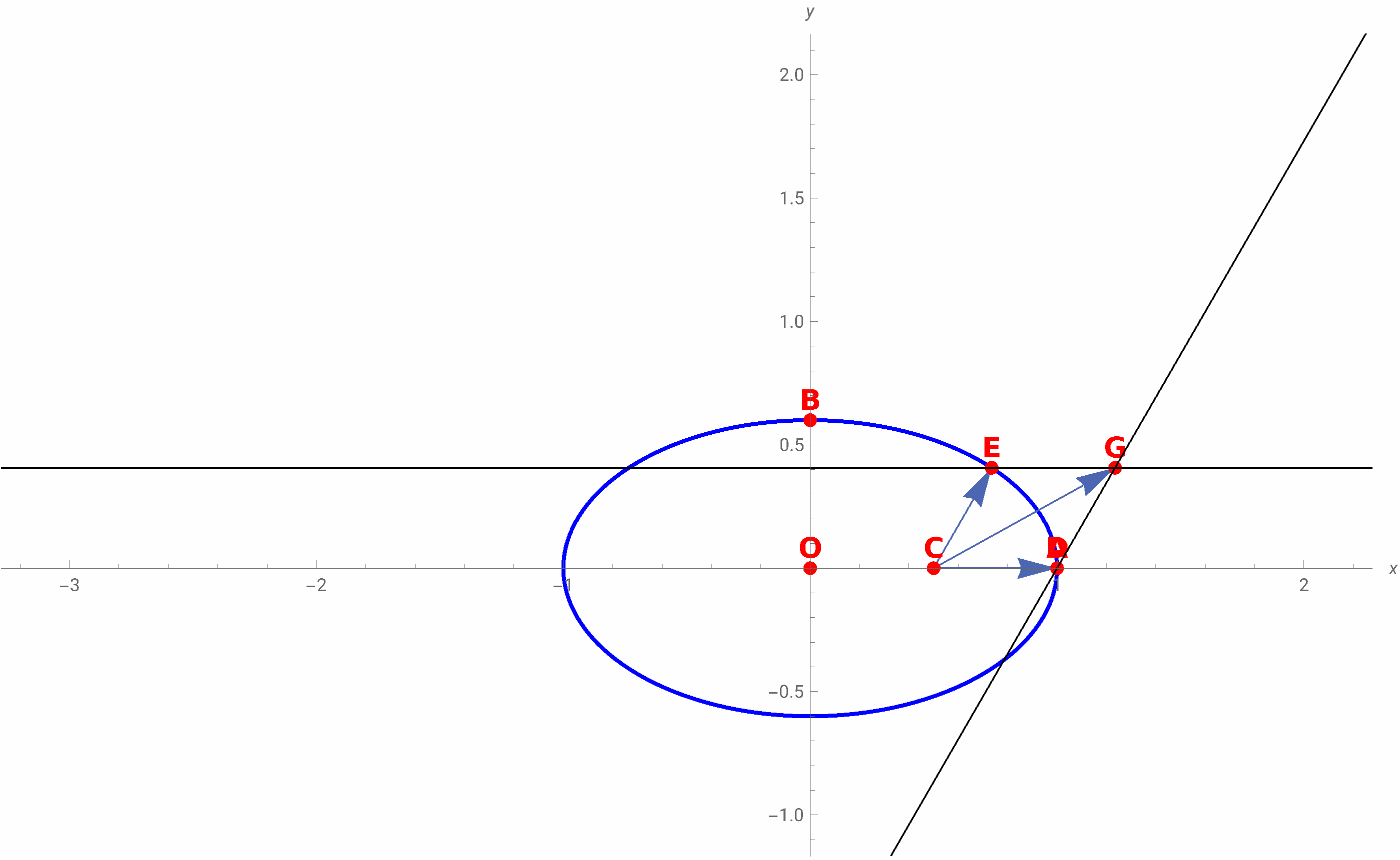
Run only the animation
In[]:=
Development:
Parametric equations of the geometric locus of G point, considering the ellipse equation +=1 .Let = k, then:
2
x
2
a
2
y
2
b
CD
In[]:=
D=={c+kCos[φ],kSin[φ]};Solve+==1,k//FullSimplify
2
(c+kCos[φ])
2
a
2
(kSin[φ])
2
b

Out[]=
k,k
-0.5Cos[φ]-0.204124
37.-13.Cos[2.φ]
1.88889-0.888889Cos[2φ]
-0.5Cos[φ]+0.204124
37.-13.Cos[2.φ]
1.88889-0.888889Cos[2φ]
In[]:=
k-,k;
b2bcCos[φ]++-+(-++)Cos[2φ]
2
a2
a
2
b
2
c
2
a
2
b
2
c
2(+)
2
b
2
Cos[φ]
2
a
2
Sin[φ]
b-2bcCos[φ]++-+(-++)Cos[2φ]
2
a2
a
2
b
2
c
2
a
2
b
2
c
2(+)
2
b
2
Cos[φ]
2
a
2
Sin[φ]
In[]:=
k[φ_]:=;
b-2bcCos[φ]++-+(-++)Cos[2φ]
2
a2
a
2
b
2
c
2
a
2
b
2
c
2(+)
2
b
2
Cos[φ]
2
a
2
Sin[φ]
Let = l, then:
CE
In[]:=
E=={c+lCos[φ+β],lSin[φ+β]};Solve+==1,l//FullSimplify
2
(c+lCos[φ+β])
2
a
2
(lSin[φ+β])
2
b
Out[]=
l,l
-0.5Sin[0.523599-1.φ]-0.204124
37.+13.Sin[0.523599+2.φ]
1.88889+0.888889Cos[1.0472-2.φ]
-0.5Sin[0.523599-1.φ]+0.204124
37.+13.Sin[0.523599+2.φ]
1.88889+0.888889Cos[1.0472-2.φ]
In[]:=
l-cCos[β+φ]++(a-c)(a+c)+,l-cCos[β+φ]++(a-c)(a+c)+;
2
b
2
a
2
b
2
Cos[β+φ]
2
Sin[β+φ]
2
a
2
b
2
b
2
Cos[β+φ]
2
a
2
Sin[β+φ]
2
b
2
a
2
b
2
Cos[β+φ]
2
Sin[β+φ]
2
a
2
b
2
b
2
Cos[β+φ]
2
a
2
Sin[β+φ]
In[]:=
l[φ_]:=-cCos[β+φ]++(a-c)(a+c)+;
2
b
2
a
2
b
2
Cos[β+φ]
2
Sin[β+φ]
2
a
2
b
2
b
2
Cos[β+φ]
2
a
2
Sin[β+φ]
In both cases k and l, the positive roots were chosen (because they are magnitudes).
Animation:
In[]:=
Manipulatea=1;b=0.6;c=0.5;β=;C1={c,0};A={a,0};B={0,b};O1={0,0};ζ[θ_]:={aCos[θ],bSin[θ]};k[φ_]:=;l[φ_]:=-cCos[β+φ]++(a-c)(a+c)+;D1[φ_]:={c+k[φ]Cos[φ],k[φ]Sin[φ]};E1[φ_]:={c+l[φ]Cos[φ+β],l[φ]Sin[φ+β]};G[φ_]:=D1[φ]+E1[φ]-C1;CD[φ_]:=D1[φ]-C1;CE[φ_]:=E1[φ]-C1;CG[φ_]:=G[φ]-C1;δ=ResourceFunction["PlotVector"][{CD[φ],CE[φ],CG[φ]},C1];Show[{ParametricPlot[ζ[θ],{θ,0,2π},PlotStyle{Blue,Thick}],ParametricPlot[G[θ],{θ,0,φ},ColorFunction->"BlueGreenYellow"],δ,Graphics[{Red,PointSize[0.01],Point[O1],Text[Style["O",14,Bold],O1,{0,-1.2}],Point[A],Text[Style["A",14,Bold],A,{0,-1.2}],Point[B],Text[Style["B",14,Bold],B,{0,-1.2}],Point[C1],Text[Style["C",14,Bold],C1,{0,-1.2}],Point[D1[φ]],Text[Style["D",14,Bold],D1[φ],{0,-1.2}],Point[E1[φ]],Text[Style["E",14,Bold],E1[φ],{0,-1.2}],Point[G[φ]],Text[Style["G",14,Bold],G[φ],{0,-1.2}],{Black,InfiniteLine[{E1[φ],G[φ]}],InfiniteLine[{D1[φ],G[φ]}]}}]},AspectRatioAutomatic,AxesTrue,AxesOrigin{0,0},AxesLabel{x,y},PlotRange{{-3,2},{-1,2}},ImageSize700],Style["Geometric locus of G point",Bold,Large],{{φ,0.00002,"Value (φ)"},0.000001,2π,0.00001},ControlPlacementTop,SaveDefinitions->True
π
3
b-2bcCos[φ]++-+(-++)Cos[2φ]
2
a2
a
2
b
2
c
2
a
2
b
2
c
2(+)
2
b
2
Cos[φ]
2
a
2
Sin[φ]
2
b
2
a
2
b
2
Cos[β+φ]
2
Sin[β+φ]
2
a
2
b
2
b
2
Cos[β+φ]
2
a
2
Sin[β+φ]
Out[]=