Highly complex behavior can emerge from remarkably simple rules. This phenomenon is exemplified by nestedly recursive functions, which are functions defined on the integers where computing a value requires computing the function at another input determined by the function itself. This project specifically studies nestedly recursive functions belonging to the “subtract-like” (S) Family, characterized by their recursive definitions involving subtraction. Using evaluation graphs, error plots, and computational experiments, the asymptotic growth, deviations from predicted behavior, and sensitivity to changes in initial conditions of these functions are analyzed. The results suggest that the deviation at each step is influenced by previous values of the function, causing deviations to propagate through the recursion. This supports the observation of the emergence of periods of calm where the function remains close to its predicted trend line, and subsequent regions of bursts where deviations are amplified.
Introduction
Introduction
Recursion is a fundamental concept in mathematics and computer science in which a function makes calls to itself, typically used to break a larger problem down into smaller sub problems. Many well-known sequences are generated recursively. For example, the Fibonacci sequence defined by = 1 is a function where each term after the initial two depends on the two preceding terms.
F[n] = F[n-1] + F[n-2] and F[0] = F[1]
A special class of recursive functions called “nestedly recursive,” termed by Stephen Wolfram, takes this idea further. We call a function nestedly recursive if the function calls itself inside its own body and that function uses the function itself as an argument. For instance, the function is nestedly recursive. Although these functions appear to have a simple form at first glance, they can generate surprisingly complex patterns that are difficult to predict.
f[n] = f[f[n-1]]
Families of Nestedly Recursive Functions
Families of Nestedly Recursive Functions
Nestedly recursive functions can be broadly categorized into three main families based on the main arithmetic operator, namely, the P, T, and S families. They stand for plus-like, times-like, and subtract-like, respectively. Though they have similar structures, functions belonging to these different families exhibit significant variations in their behavior. This project focuses on the lesser-explored S Family functions, including their evaluation graphs, asymptotic behavior, and what happens when the function definition changes.
The basic structure of a nested recursive function belonging to the “subtract-like” or S Family is of the form . Let the initial condition be for all n ≤ c. Such a function is denoted by . By varying these parameters, this project aims to explore how the structure and long-term behavior of S Family functions change.
f[n] = n – f[f[n – a] – b]
f[n] = 1
Sab
The S Family
The S Family
A Basic Example
A Basic Example
Consider the function (), which is also known as the Hofstadter G-Sequence. In this example, the initial condition f[n] = 1 for will be used. (Note that using f[n] = 0 for n ≤ 1 leads to the circular definition ).
S10
S1
n ≤ 1
f[1] = f[1]
f[n_/;n>1]:=n-f[f[n-1]];f[n_/;n<=1]:=1
We can define such a recursive function using the ResourceFunction[“RecursiveFunction”] from the Wolfram Function Repository.
This function computes a list of () up to the nth term, where the number of terms is specified by the parameter . accepts the inputs or and recursively evaluates the function over the given integer input(s):
f[n]
Sab
steps
ResourceFunction["RecursiveFunction"]
[fun, inits, n]
[fun, inits, {n1,n2,…}]
In[]:=
f[a_:1, b_:0, c_:1, steps_] := ResourceFunction["RecursiveFunction"]f.[n.] -> n. - f.f.[n. - a] - b, {n. <= c -> 1}, Range[steps]
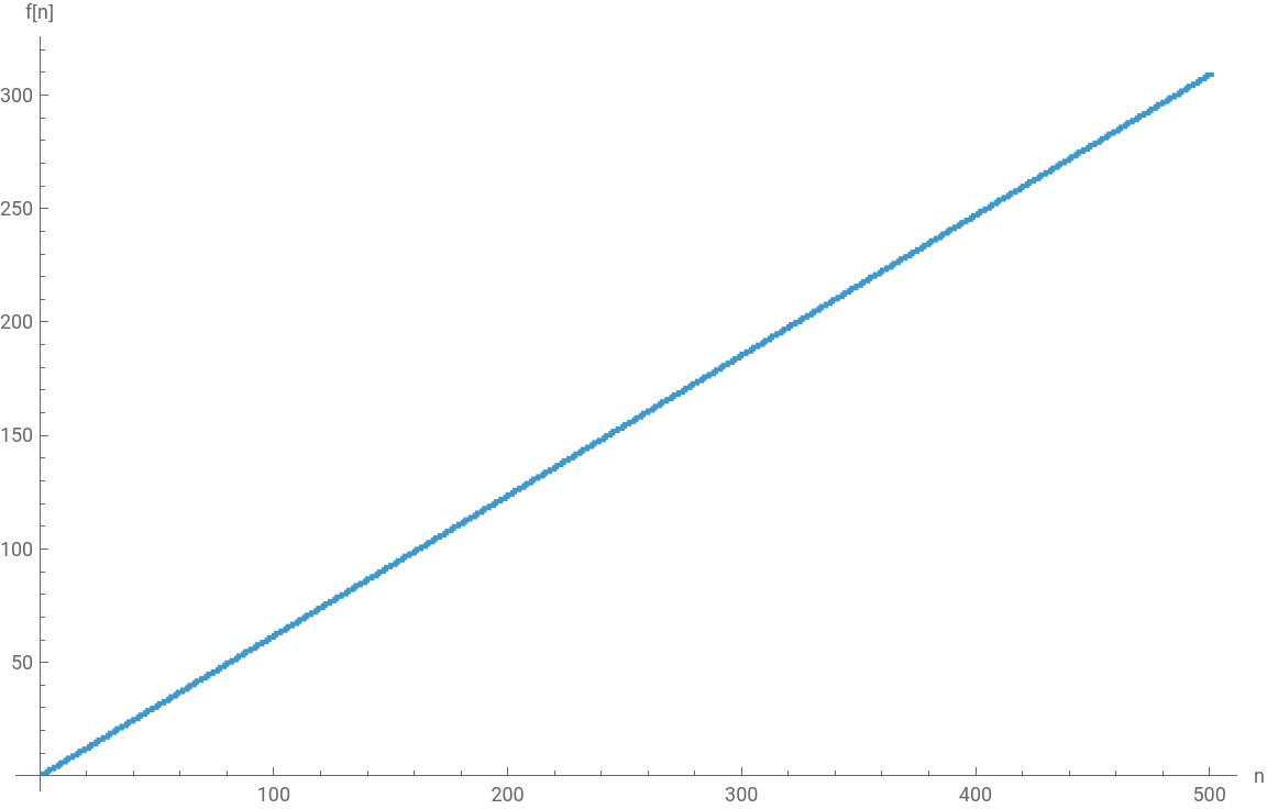
Compute a list of up to the 500th term:
f[n]
In[]:=
Short[data=f[500]]
Out[]//Short=
{1,1,2,3,3,4,4,5,6,6,7,8,8,9,9,10,11,11,12,12,13,14,14,15,16,450,294,295,296,296,297,297,298,299,299,300,300,301,302,302,303,304,304,305,305,306,307,307,308,309,309}
An animation of for the first 500 values:
f[n]
In[]:=
AnimateListStepPlotdata[[;;n]],,{n,1,500,1},
Out[]=
Evaluation Graphs
Evaluation Graphs
Function calls can be traced using an evaluation graph (generated by ), which gives a visualization for each successive function call a function leads to. Each vertex represents a function evaluation, and the arrows serve as directed edges that point to the next function call that is made. As a result, evaluation graphs provide an intuitive way to understand how recursive functions are computed.
ResourceFunction["RecursiveFunctionCallGraph"]
For a simple example, the call graph of the Fibonacci sequence is shown below:
ManipulateResourceFunction["RecursiveFunctionCallGraph"]f.[n.]->f.[n.-1]+f.n.-2,{n.<=1->1},steps,,{{steps,5},1,10,1},
Out[]=


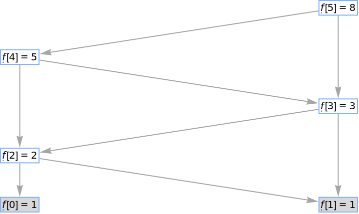
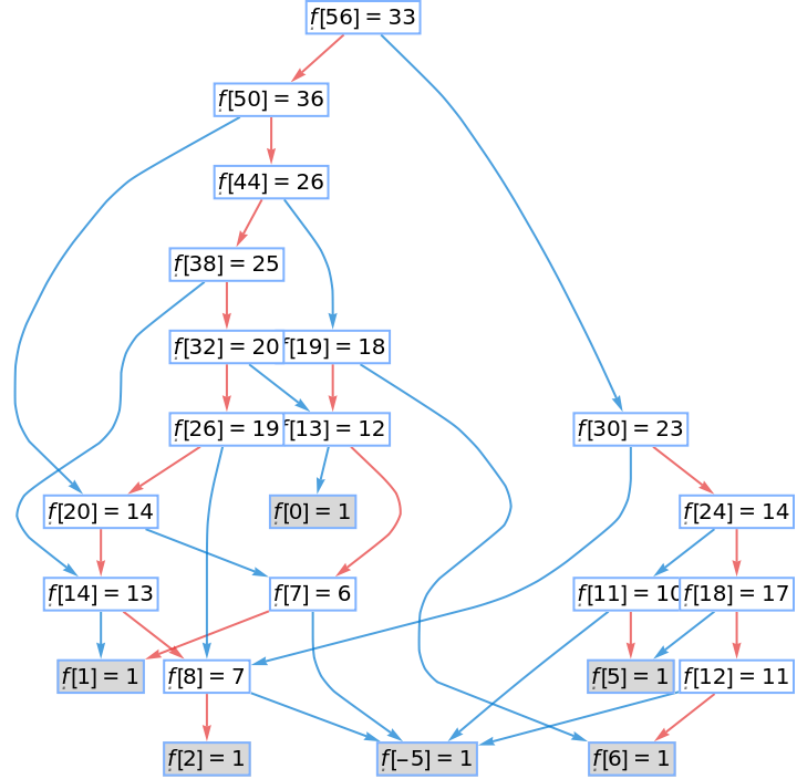
Evaluation graphs are especially useful for keeping track of function calls in the nested case, where the graphs become much more complicated due to the presence of recursive calls within recursive calls. To distinguish between the two levels of recursion, calls made from the inner function will be denoted with a red arrow, while calls from the outer function will be denoted with a blue arrow.
Calls are color-coded for clarity — calls from the inner function will use red arrows, calls from the outer function will use blue arrows:
In[]:=

Out[]=
f.[n._] := n.-
In the graph below, shaded boxes represent the initial values needed for the computation, corresponding to where was sampled for . Note that not all base values are referenced for a computation, indicating that only a subset of possible base cases actually contributes to the computation. This will be explored later in greater detail.
f[n]
n≤c
Using , the values of a, b, and c in the initial condition f[n] = 1 for n ≤ c can be changed. Code adapted from Stephen Wolfram’s “Nestedly Recursive Functions”:
Manipulate
ManipulateLabeledResourceFunction["RecursiveFunctionCallGraph"]f.[n.]n.-f.f.[n.-a]-b,{n.≤c1},steps,Sequence[GraphLayout"LayeredDigraphEmbedding","AddFigures"True,EdgeStyle{x_<|1,2|>[Last[x]]},AspectRatio1],Sequence,{a,1,9,1},{b,0,9,1},{c,1,9,1},{{steps,10},1,100,1},
Out[]=
To take a closer look, the evaluation graph can be decomposed into its “red” and “blue” subgraphs. For the red graph, each node points to ,representing the inner recursive call in the definition of the Sab function.
n
n-a
Red (inner) graph:
ManipulateLabeledRow@ResourceFunction["RecursiveFunctionCallGraph"]f.[n.]->n.-f.f.[n.-a]-b,{n.<=c->1},steps,,1,,{{a,1},1,9,1},{{b,0},0,9,1},{c,1,9,1},{{steps,8},1,100,1},
Out[]=
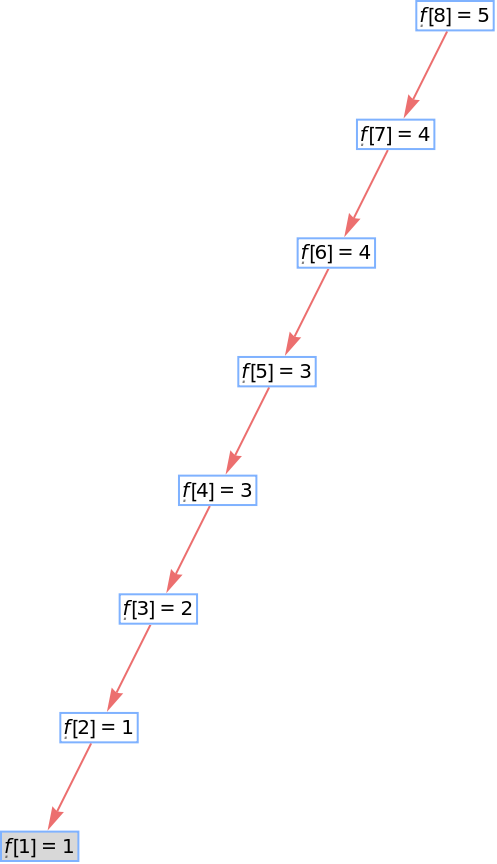
In contrast to the linear red graph, the blue graph has a more tree-like structure, where each tree terminates at a separate initial condition.
Blue (outer) graph:
Finding Asymptotic Behavior
Finding Asymptotic Behavior
Plots with different values for a and b are shown below (initial condition remains unchanged):
Interestingly, the error plot reveals what appears to be "regions of calm" followed by "bursting" behavior. During the calm regions, the function remains relatively close to its predicted asymptotic trend, but experiences larger amplified deviations during the burst intervals. This raises several questions: What characteristics of the function causes this bursting behavior? Do they occur at predictable intervals?
Extracting Burst Intervals
Extracting Burst Intervals
To better visualize the distinction between “burst” versus “calm” intervals observed in the error plot, they will next be plotted separately in this section. By isolating these two types of behaviors, it becomes easier to identify the underlying patterns. This analysis focuses specifically on S1 with the initial condition f[n] = 1 for n ≤ 3, as that is when the bursting behavior is first observed.
Getting the sequence:
Define a threshold for the error:
Helper method that will use the list from burstQ to separate intervals based on whether or not they are bursts:
Extract intervals where there are bursts:
Extract intervals which are calm:
Plot only calm points:
Plot only burst points:
Separating the burst and calm regions makes it clear that the irregularity of the error sequence is not uniformly distributed.
Scaling of Calm Regions
Scaling of Calm Regions
In the graphs above, the lengths of each successive calm interval appears to grow exponentially instead of increasing by a constant amount each time. This raises the possibility that the scaling might follow a consistent factor. To investigate this, the lengths of the calm intervals are measured and compared to determine whether they approach a constant ratio between successive intervals.
Get the length of each calm interval:
Make a list of each calm interval followed by the length of that interval:
The table below displays when a calm interval starts, ends, and its length:
Random, short-term fluctuations (i.e., intervals with minimal lengths) can obscure the overall scaling factor and should therefore be ignored for the analysis. Hence, only the longest, “record-breaking” calm lengths will be extracted and analyzed. This allows for the asymptotic growth ratio to be analyzed more accurately.
Gets the indices of where each largest calm interval starts (refer to the table above):
Extract the intervals at those indices:
Extract the lengths at those indices:
Now that the lengths of each successive region of calm have been extracted, the ratio of the length between consecutive intervals can be calculated to find the scaling factor.
Compute each successive ratio:
Display them in a table:
Deriving Error Formula
Deriving Error Formula
Testing Bursting
Testing Bursting
Define the function:
Define the error:
The boolean pairs are then counted to determine how frequently each combination occurs:
Display data in a table:
Next, extract the values we are looking for, which are the cases where a burst was observed at n .
Display values in a table:
Getting the ratio:
Changing Parameters
Changing Parameters
More with Evaluation Graphs
More with Evaluation Graphs
The general shapes and topology of the evaluation graphs can be visualized when the number of steps is increased to a much larger value.
Here is the evaluation graph for S1 with 300 steps:
A three-dimensional visualization provides another perspective on the evaluation graph. As shown below, the graph of S1 forms a surface resembling a hyperbolic paraboloid.
3D graph of S1 with 2000 steps:
Graph Analysis
Graph Analysis
Create a list of graphs to be analyzed. The value of a goes from 1 to 10, the value of b goes from 0 to 10:
Average of the number of edges for each value of a:
Average of the number of vertices for each value of a:
GraphDensity measures ratio of the number of edges divided by the number of edges of a complete graph with the same number of vertices.
Normalizing the densities:
Analyzing Deviations
Analyzing Deviations
Plots of the absolute difference for different S functions:
Examining the scale of the vertical axis reveals that the absolute value of the deviation increases with greater values of a and b, suggesting that larger parameters introduce greater fluctuations from the expected asymptotic behavior. Additionally, there seems to be some periodic behavior where the error increases and decreases.
Changing Initial Conditions
Changing Initial Conditions
Error plot for S1 with different initial conditions:
Here, there error seems to follow a much simpler and more predictable pattern, where it expands outward in a triangular shape. To better understand the source of these patterns, it is useful to go back to evaluation graphs to examine how the behavior is affected by initial conditions.
Function that takes in the parameters a, b, c for the function definition and plots the points up to n = 100 in the color corresponding to which tree the point belonged to:
Plots for S functions with different parameter values and initial conditions. Initial conditions are color-coded to indicate the number of initial conditions referenced for a computation:
In the Manipulate below, the initial condition can be changed for each S function:
S11 with initial condition f[n] = 1 for n ≤ 3:
After the first few initial terms, this sequence alternates between the sequence of odd integers and the constant value 4. In fact, the graph above shows that S11 has this “alternating” behavior for any initial condition f[n] =1 for n ≤ c where c ≥ 3. For example, below is S11 with initial condition f[n] =1 for n ≤ 4, which follows a very similar pattern.
S11 with initial condition f[n] = 1 for n ≤ 4:
Besides S11, S13 and S15 also have the alternating pattern starting from f[n] = 1 for n ≤ 3 as the initial condition.
S13 with initial condition f[n] = 1 for n ≤ 4 :
Plotting the error for S13 with different initial conditions reveals that it follows a similar pattern to S11 where after the initial condition f[n] = 1 for n ≤ 3, a triangular shape appears.
When the initial condition is changed to f[n] = 1 for n ≥ 4, S23 also begins to exhibit this alternating behavior. The error plot below supports the idea that this alternating pattern is responsible for the triangular structure of the error. In particular, notice that the triangular pattern begins at n = 4, which is the same point where the alternating pattern appears in the sequence.
Overall, these results reveal an interesting pattern that appears for certain combinations of parameters and initial conditions. In these cases, the triangular shape of the error seems to be caused by the emergence of a constant term that alternates between values in the sequence. Although the specific parameters that produce these conditions was not analyzed due to the time constraint, the presence of this pattern illustrates the complex relationship between parameters, initial conditions, and the resulting asymptotic behavior of the function.
Conclusion
Conclusion
Future Directions
Future Directions
1. Analysis of initial conditions can be extended to more rigorously analyze the the emergence, frequency, and magnitude of bursting behavior in the error function.
2. On the mathematical side, future work could focus on connecting computed observations to the underlying definitions of the function.
3. Extend the analysis to other families of nestedly recursive functions.
2. On the mathematical side, future work could focus on connecting computed observations to the underlying definitions of the function.
3. Extend the analysis to other families of nestedly recursive functions.
References
References
◼
Wolfram, S. (2024, September 27). Nestedly Recursive Functions. Stephen Wolfram Writings. https://writings.stephenwolfram.com/2024/09/nestedly-recursive-functions/
◼
Klee, B., & Adler, T. (2024, September 16). RecursiveFunction. Wolfram Function Repository. https://resources.wolframcloud.com/FunctionRepository/resources/RecursiveFunction
◼
Klee, B., & Adler, T. (2024, September 23). RecursiveFunctionCallGraph. Wolfram Function Repository. https://resources.wolframcloud.com/FunctionRepository/resources/RecursiveFunctionCallGraph/
◼
OEIS Foundation Inc. (2026). Hofstadter G-sequence. The On-Line Encyclopedia of Integer Sequences. https://oeis.org/A005206
Acknowledgements
Acknowledgements
First, I would like to express my gratitude to my mentor, Daniel Sanchez, for guidance, expertise, and support throughout the entirety of this project. His patience in helping to debug my code, insightful suggestions, and ability to keep me on task were essential to the completion of this project. I would also like to thank Stephen Wolfram for laying out the foundations of this project and helping shape the direction of my ideas. Lastly, I would like to thank Rory Foulger, Eryn Gillam, and Megan Davis for running this program and providing this opportunity to me.
Additional thanks to Stephen Wolfram for suggesting this project.
CITE THIS NOTEBOOK
CITE THIS NOTEBOOK
Analyzing properties and behaviors of S family nestedly recursive functions
by Gracelyn Chen
Wolfram Community, STAFF PICKS, July 9, 2026
https://community.wolfram.com/groups/-/m/t/3752960
by Gracelyn Chen
Wolfram Community, STAFF PICKS, July 9, 2026
https://community.wolfram.com/groups/-/m/t/3752960