Here is the whole story in a few lines. We start with the cubic curve and the rational point . Repeatedly intersecting the curve with tangent lines produces new rational points, and ToWeierstrass carries all of them over to the Weierstrass normal form.
f=0
P=(1,1)
In[]:=
f=+2-7xy+4;points=NestList[GenerateNextPoint[f,{x,y},#]&,{1,1},6];weierstrass=ToWeierstrass[f,{x,y},{1,1}];weierstrass["Curve"]//TraditionalForm
3
x
3
y
Out[]//TraditionalForm=
2
y
3
x
In[]:=
ComparisonPlot[f,{x,y},weierstrass,points]
Out[]=
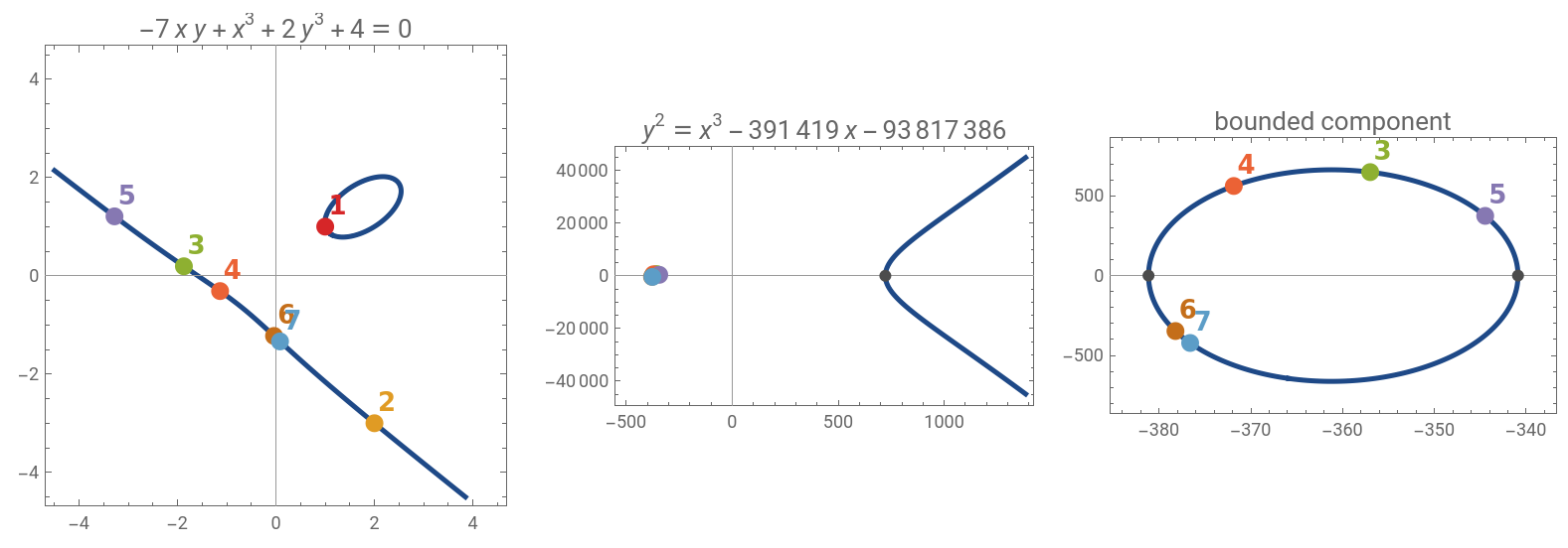
On the left you see the original curve with the base point (number 1, red) and the points 2, 3, ... that the tangent construction generates from it. In the middle you see the Weierstrass curve, on the right a zoom onto its bounded component. The base point (1) is sent to the point at infinity. The point (2) is the third intersection of the tangent at , which is mapped to the line at infinity, so the formula for the map breaks down there too, and the point is missing in the plots; its actual image, however, is a finite point on the oval. Every other point lands on the oval.
P
Q
P
The returned association contains more than the curve:
In[]:=
KeyDrop[weierstrass,"Map"]
Out[]=
Curve-93817386-391419x+,A-391419,B-93817386,Discriminant35671071454101504,j,FlexFalse
2
y
3
x
3046733141473
16387064
My personal plan is to dig deeper into elliptic curves. These are my notes after reading the first chapter of Silverman and Tate. If you find these notes useful and want me to keep writing up what I learn about elliptic curves, leave a like or a comment. If you think I’m spamming the Wolfram Community, let me know as well :-).
Introduction: From Ten to Two Coefficients
Introduction: From Ten to Two Coefficients
A general cubic curve in the plane is the zero set of a polynomial of degree three in and . It has ten coefficients :
x
y
α
i
In[]:=
EC:=+x+y+++xy++y+x+;
α
1
3
y
α
2
2
y
α
3
2
x
α
4
3
x
α
5
2
y
α
6
α
7
2
x
α
8
α
9
α
10
Since the equation can be multiplied by any non-zero number, only nine of them really count. A smooth curve with a rational point is an elliptic curve. Number theorists are mainly interested in its rational points, the pairs that satisfy the equation. By Mordell’s theorem, these points form a finitely generated abelian group.
EC=0
(x,y)∈
2
ℚ
The structure of the set of rational points does not change when we perform a change of variables that is defined over the rationals and can be inverted (a birational transformation): rational points go to rational points and back. We can use such transformations to simplify the appearance of the curve. The goal is the Weierstrass normal form
2
y
3
x
which depends on only two parameters. Even these two are not unique: the scaling changes and leaves the -invariant
(x,y)x,y
2
u
3
u
(A,B)(A,B)
4
u
6
u
j
j=
1728(4)
3
A
4+27
3
A
2
B
unchanged. Over the complex numbers, alone determines the curve up to isomorphism.
j
There is one important requirement: we need a rational point on the curve to start with. Without it, the method does not work, and there are smooth cubics with no rational point at all, for instance Selmer's curve [3]. Such a curve is not isomorphic to any Weierstrass curve over .
P
3+4+5=0
3
x
3
y
ℚ
We follow the construction of Silverman and Tate [1]. It consists of the following steps:
◼
Pass to the projective plane, where all lines meet and points at infinity are ordinary points.
◼
Move the rational point to (a point on the line at infinity), and its tangent line to (the line at infinity).
P
(1:0:0)
Z=0
◼
Move the third intersection of that tangent with the curve to and the tangent at to .
Q
(0:1:0)
Q
X=0
◼
Return to the affine plane (the familiar ) and apply a quadratic transformation that turns the curve into +(ax+b)y=c+d+ex+g.
2
2
y
3
x
2
x
◼
Complete the square, normalize the cubic and remove its quadratic term.
◼
Rescale to integral and minimal coefficients.
The post contains seven sections:
1
.We first show how a sequence of rational points can be generated from a single rational point.
2
.In the next section, we describe the necessary steps that turn an arbitrary elliptic curve into Weierstrass form. The transformation of an explicit example curve illustrates the description and makes this section rather technical. You might want to skim it on a first read and only collect the geometric interpretations of the transformations.
3
.These geometric properties are visualized in the third section. Since points at infinity and the line at infinity play a major role in the discussion of these steps, the visuals are presented in two panels. One holds a hemisphere that represents a projection of the entire projective plane. The second panel shows the traditional -plane, which the text calls the affine chart at .
2
Z1
4
.The next section shows yet another example, the famous taxicab curve.
5
.The presented recipe is generic. To show this, you can explore random elliptic curves with a rational point and observe the action of ToWeierstrass, which bundles all the steps into a single function.
6
.The last part explains the function ToWeierstrass in detail.
7
.The post closes with the code that is used inside the notebook (most of it is vibe-coded) and the references.
Rational Points from Tangents
Rational Points from Tangents
A line meets a cubic curve in three points (counted with multiplicity and possibly at infinity). If two of them are rational, the third one has to be rational, too. For the tangent at a rational point this is especially useful: counts twice, so the third intersection is a new rational point. Let us compute it for our curve and . The tangent is obtained from the first order Taylor expansion (the zeroth-order term vanishes, since ):
P
P
f=+2-7xy+4
3
x
3
y
P=(1,1)
f(P)0
In[]:=
P={1,1};gradient=D[f,{{x,y}}]/.Thread[{x,y}->P]tangentLine=Expand[gradient.({x,y}-P)]==0
Out[]=
{-4,-1}
Out[]=
5-4x-y0
We walk along the tangent, , with a direction orthogonal to the gradient. When this line is substituted into the equation , it becomes a cubic polynomial in . The constant term vanishes since lies on the curve, and its linear term vanishes since the line is tangent, i.e. is a double zero ( counts as two roots):
(x,y)=P+td
d
f0
t
P
t=0
P
In[]:=
d={-gradient[[2]],gradient[[1]]};restricted=Expand[f/.Thread[{x,y}->P+td]]
Out[]=
127-127
2
t
3
t
The remaining root is rational and gives the next rational point:
t=-
c
2
c
3
In[]:=
{c2,c3}=Coefficient[restricted,t,{2,3}];Q=P-c2/c3d
Out[]=
{2,-3}
In[]:=
Show[CurvePlot[f,{x,y},{P,Q}],ContourPlot[Evaluate[tangentLine],{x,-4.5,4.5},{y,-4.5,4.5},ContourStyle->Directive[Dashed,Gray]]]
Out[]=
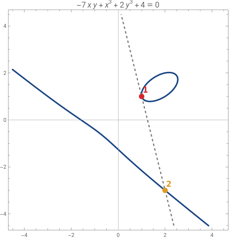
This is all that GenerateNextPoint does. If is an inflection point (a flex), then =0 and the tangent meets the curve only at ; if =0, the third point lies at infinity. Iterating the construction yields the sequence of points we have seen above:
P
c
2
P
c
3
In[]:=
points[[1;;5]]//Column
Out[]=
{1,1} |
{2,-3} |
- 58 31 6 31 |
- 860807 757733 235707 757733 |
- 1520554029210774079694038 463473097001157009316981 560531527564519577185737 463473097001157009316981 |
The numbers grow quickly. The number of digits of the denominators roughly quadruples in every step.
The Transformation Step by Step
The Transformation Step by Step
Into the projective plane
Into the projective plane
In the projective plane, a point is described by homogeneous coordinates , which are only defined up to a common factor. The affine points are , and the points with are the points at infinity. We homogenize the equation by substituting , and multiplying by :
(X:Y:Z)
(x:y:1)
Z=0
x=
X
Z
y=
Y
Z
3
Z
In[]:=
homogeneous={x->X/Z,y->Y/Z};ExpandEC/.homogeneous
3
Z
Out[]=
3
Y
α
1
2
Y
α
2
2
X
α
3
3
X
α
4
2
Y
α
5
α
6
2
X
α
7
2
Z
α
8
2
Z
α
9
3
Z
α
10
Every term now has degree three. For our example, with :
P=(::1)=(1:1:1)
x
P
y
P
In[]:=
xP=1;yP=1;homExample=Expandf/.homogeneous
3
Z
Out[]=
3
X
3
Y
3
Z
Choosing the axes
Choosing the axes
Following Silverman and Tate (Section 1.3 and Figure 1.10 in [1]), we choose new projective coordinates such that the tangent to the curve at becomes the line at infinity, the tangent at the third intersection point of this tangent with the curve becomes the vertical axis, and some other line through becomes the horizontal axis. We get there in four steps. Each step is a linear change of the homogeneous coordinates with rational coefficients. Such a change maps lines to lines, tangents to tangents and rational points to rational points.
P
Q
P
To keep track of the coordinates, we number them by the step that introduces them. The original coordinates are , and Step introduces :
(X,Y,Z)
k
(,,)
X
k
Y
k
Z
k
(X,Y,Z)(,,)(,,)(,,)(,,)
X
1
Y
1
Z
1
X
2
Y
2
Z
2
X
3
Y
3
Z
3
X
4
Y
4
Z
4
For every step we write down the new coordinates in terms of the old ones (the rules t1, t2, ...). To transform the equation, we need the inverse substitution, which expresses the old coordinates in terms of the new ones (the rules it1, it2, ...).
Step 1: Move P to (1:0:0)
Step 1: Move P to (1:0:0)
Step 3: Move the third intersection Q to (0:1:0)
Step 3: Move the third intersection Q to (0:1:0)
Four of the ten monomials are missing now, each for a geometric reason:
Step 5: A quadratic transformation
Step 5: A quadratic transformation
Step 6: Complete the square
Step 6: Complete the square
Step 7: Normalize the cubic
Step 7: Normalize the cubic
Step 8: Remove the quadratic term
Step 8: Remove the quadratic term
This is the Weierstrass normal form, but with ugly rational coefficients.
Step 9: Integral coefficients
Step 9: Integral coefficients
Step 10: Minimal coefficients
Step 10: Minimal coefficients
This is the same curve that ToWeierstrass produced at the beginning:
Visualize the Transformations on the Hemisphere
Visualize the Transformations on the Hemisphere
In the animations, we work with an elliptic curve whose coefficients stay rather small during transformation:
Besides these static images, the WeierstrassExplorer lets you watch the transformations live as they transit from the initial to the final state.
The Taxicab Curve
The Taxicab Curve
Since we know more than one rational point we have an alternative way to obtain new rational points. We can construct chords through two points and compute the third intersection with the chord. This is done with the help of the function GenerateNextPointFromChord
When this construction is iterated, make sure that you skip one point in the list, since three consecutive points always lie on the same line and would cause a cycle.
Explore It Yourself
Explore It Yourself
Inside ToWeierstrass
Inside ToWeierstrass
The function ToWeierstrass performs the same steps for any smooth cubic with rational coefficients and any rational point. The coordinate changes in Steps 1 to 4 are carried out by a small helper function.
Linear changes of coordinates
Linear changes of coordinates
The tangents
The tangents
The flex case
The flex case
Following the points
Following the points
The key "Map" holds the composition of all transformations. It maps affine points of the original curve to points of the Weierstrass curve. All images indeed satisfy the new equation:
The formula fails for the first two points:
Independence of the base point
Independence of the base point
What happens if we start from another rational point?
Error handling
Error handling
References
References
[1] J. H. Silverman and J. T. Tate, Rational Points on Elliptic Curves, 2nd ed., Undergraduate Texts in Mathematics, Springer, 2015. Section 1.3 and Appendix B.
[2] M. Artin, F. Rodriguez-Villegas and J. Tate, "On the Jacobians of plane cubics", Advances in Mathematics 198 (2005), 366–382.
[3] J. W. S. Cassels, Lectures on Elliptic Curves, London Mathematical Society Student Texts 24, Cambridge University Press, 1991.
CITE THIS NOTEBOOK
CITE THIS NOTEBOOK
Elliptic curves in Weierstrass normal form
by Johannes Martin
Wolfram Community, STAFF PICKS, October 27, 2026
https://community.wolfram.com/t/28424/
by Johannes Martin
Wolfram Community, STAFF PICKS, October 27, 2026
https://community.wolfram.com/t/28424/