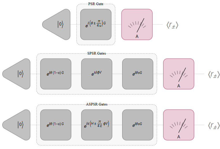
In the following example we will illustrate how to apply The Parameter Shift-Rule, The Stochastic Parameter Shift-Rule and The Approximate Stochastic Parameter Shift-Rule in order to differentiate any qubit gate.
Paclet Installation
Paclet Installation
Wolfram quantum framework is a paclet. So first, let’s install it:
PacletInstall["https://wolfr.am/DevWQCF",ForceVersionInstall->True]
In[]:=
<<Wolfram`QuantumFramework`
Defining Helper Functions
Defining Helper Functions
The Parameter-shift rule
The Parameter-shift rule
Theory
Theory
The expected value of a circuit in relation to a measurement operator varies smoothly with the circuit’s gate parameters θ. This expected value can be expressed as . This implies that the derivatives 〈A〉 are well–defined, allowing for the application of gradient descent.
A
〈A(θ)〉
∇
θ
Even though a circuit might have numerous gates, our focus can be on a single gate for differentiation
Out[]=
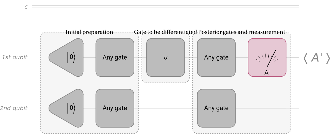
All gates preceding the specific gate of interest can be incorporated into an initial state and all posterior gates to an effective measurement operator A.
|〉
ψ
0
Out[]=
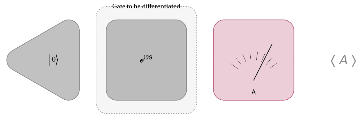
Any unitary gate can be cast in the form , where is the Hermitian generator of the gate . And the expectation value is the same as the expectation value .
U=
iθG
e
G
U
〈A〉
〈A'〉
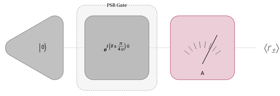
The parameter–shift rule states that in order to obtain the derivative 〈A〉 from gate we need to compute:
∇
θ
U
Out[]=
∇
θ
π
4u
π
4u
where is an arbitrary real number, that we will take equal to .
u
1/2
Example
Example
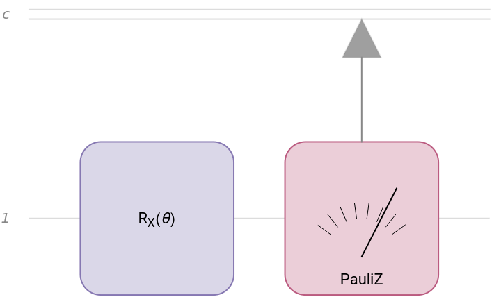
We will consider a circuit in which the gate (θ) will be differentiated:
R
x
In[]:=
RXCircuit=QuantumCircuitOperator[{"RX"[θ],QuantumMeasurementOperator["PauliZ"->{-1,1}]},"Parameters"->{θ}];
In[]:=
RXCircuit[θ]["Diagram",ImageSize->Medium]
Out[]=
The following function can obtain the symbolic expected value for our measurement:
In[]:=
RxExpectedValue[θ_]=RXCircuit[θ][]["Mean"]//ComplexExpand//Simplify
Out[]=
Cos[θ]
Calculating and , we compute the gradient of (θ):
〈〉
r
+
〈〉
r
-
R
x
In[]:=
RxParameterShiftGradient=(RxExpectedValue[θ+π/2]-RxExpectedValue[θ-π/2])//Simplify
1
2
Out[]=
-Sin[θ]
The parameter–shift rule only works for gates of the form where =1, in other cases that does not fulfill these conditions, the stochastic parameter–shift rule must be used.
θG
2
G
The Stochastic Parameter-shift rule
The Stochastic Parameter-shift rule
Theory
Theory
In contrast with the regular method, the stochastic parameter-shift rule (SPSR) adds a random parameter s and one additional gate on each side.
If G is the generator of the gate U we are about to differentiate, we first express as a sum of tensor product of Pauli operators , where is a tensor product of Pauli operators and H represents any linear combination of tensor products involving Pauli operators, chosen arbitrarily.
G
G=H+θV
V
The SPSR algorithm require us to implement the following 3 gates:
Out[]=
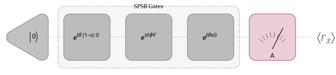
where s is a uniform random variable in the interval , which we will be sampling multiple times for each θ. The expected value of this circuit will be called or depending on the ϕ shift sign. The gradient can be obtained from the average:
[0,1]
〈〉
r
+
〈〉
r
-
∇
θ
Ε
sϵ[0,1]
r
+
r
-
Example on a cross–resonance gate
Example on a cross–resonance gate
The Approximate Stochastic Parameter-shift rule
The Approximate Stochastic Parameter-shift rule
Theory
Theory
The implementation of gates with form for the SPSR algorithm could pose challenge for some hardware. In order to address that problem we can implement the Approximate Stochastic Parameter-shift rule (ASPSR):
±V
π
4
In contrast with the regular SPSR we got some extra terms ϵ and H in the sandwiched gate:
Out[]=
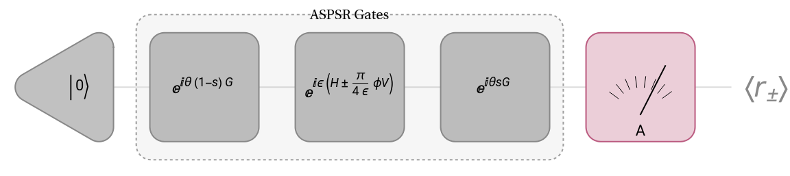
In this example , we will assume . The gradient can be obtained from the average:
ϵ=
π
4
Example on a cross–resonance gate
Example on a cross–resonance gate
The implementation of a single ASPSR circuit would be the following:
First we need to implement the H operator from our generator:
Now we can define the circuit:
Since the calculation is basically the same compared to the standard SPSR algorith, we will directly use the function ASPSRGradientValues to compute the gradient, which needs the same input than the SPSR version but including the H operator:
Lets plot it along with the previous result:
We can verify their match using Fourier interpolation:
Acknowledgment
Acknowledgment
I would like to express my sincere gratitude to Cesar Guerra and the Wolfram Quantum Computation Framework Team for their help through this notebook implementation.
References
References
Banchi, L., & Crooks, G. E. (2021). Measuring Analytic Gradients of General Quantum Evolution with the Stochastic Parameter Shift Rule. In Quantum (Vol. 5, p. 386). Verein zur Forderung des Open Access Publizierens in den Quantenwissenschaften. https://doi.org/10.22331/q-2021-01-25-386
Killoran, N. (2020). The stochastic parameter-shift rule. PennyLane Demos. https://pennylane.ai/qml/demos/tutorial_stochastic_parameter_shift/
CITE THIS NOTEBOOK
CITE THIS NOTEBOOK
Parameter Shift-Rule to Differentiate Qubit Gates: Stochastic and Approximate Stochastic Algorithms
by Sebastian Rodriguez
Wolfram Community, STAFF PICKS, February 28, 2024
https://community.wolfram.com/groups/-/m/t/3132207
by Sebastian Rodriguez
Wolfram Community, STAFF PICKS, February 28, 2024
https://community.wolfram.com/groups/-/m/t/3132207