Wolfram Cloud Document

Cancer treatment and its interaction with the human body is not well-understood by the general population and even some cancer patients but understanding it is essential for improving cancer treatment strategies. This study focuses on demystifying and developing a series of mathematical models, from classic tumor-immune ODEs to extended delay differential systems incorporating chemotherapy and drug-resistant tumor populations. Through simulations, biomarker analysis, and multi-objective optimization, we demonstrate how resistance emerges, how immune-tumor dynamics evolve, and how adaptive dosing protocols may outperform static ones. The results emphasize the importance of incorporating resistance mechanisms , patient-specific biomarkers in optimizing cancer therapies, and dynamic regimens are necessary for successful tumor control.

Introduction

Why Modeling Tumor-Immune Dynamics Matters

Cancer is one of the leading causes of death worldwide and one of the most common diseases. However, the immune system is able to fight off and identify potential cancers, often successfully, without us even realizing it. So, a key reason why cancer is so deadly is that cancer cells, also known as tumors, often adapt by suppressing immune responses or evolving resistance to treatment, allowing them to grow unchecked. The most common cancer treatment is chemotherapy, the use of drugs that kill both tumor and normal cells in the body with the hope that the tumor cells will be killed off before the normal ones. While initially effective, chemotherapy frequently leads to the emergence of drug-resistant tumor cells, a subpopulation that survives treatment and repopulates the tumor. Finding more effective alternatives to chemotherapy for cancer treatment have been hampered by the complexity of tumor-immune interactions and the emergence of drug resistance by tumors. Recent advances in drug-delivery research further highlighted the importance of treating delivery mechanisms as an active variable rather than a passive component of therapy. Professor Shaoyi Jiang’s work on zwitterionic-polymer-coated lipid nanoparticles demonstrated that carefully engineered delivery vehicles can dramatically reduce immunogenicity and improve therapeutic stability in cancer vaccines. His findings showed that material-science innovations directly influence immune activation, treatment resistance, and overall therapeutic efficacy. Because of this, I incorporated chemotherapy delivery dynamics explicitly into my model, treating drug exposure, toxicity, and immune interaction as mathematically significant processes rather than background assumptions. As experimental approaches to study these dynamics are costly and time-consuming, computational modeling offers an efficient and insightful way to explore complex biological behavior and communicate the results in a straightforward way.

Project Objectives

Begin with the Kuznetsov et al. ODE model of tumor-immune interaction, extend it using Rihan et al.’s delay differential equations (DDEs), and incorporate chemotherapy and tumor resistance.

Simulate the evolution of drug-resistant tumor cells under chemotherapy and assess how treatment timing and intensity impact resistance dynamics.

Define and track both primary and composite biomarkers, such as immune efficiency, tumor burden, resistance fraction, and survival index to assess treatment progress and prognosis.

Evaluate and compare different chemotherapy strategies (continuous, intermittent, and adaptive) using multi-objective Pareto optimization targeting tumor suppression, immune preservation, and toxicity minimization.

Use Monte Carlo simulations to quantify uncertainty in final tumor burden under random biological variability.

Implement correlation matrices to understand further the relationships between cell populations.

Original Tumor-Immune Models

We will start by modeling cancer dynamics with just the immune system as a defense, before extending the simulation with chemotherapy.

Explanation of Model

We begin without chemotherapy in order to understand tumor-immune dynamics before adding another variable into the mix. For this, we use Kuznetsov et al.’s model that accomplishes this by incorporating a system of five ordinary differential equations. The model describes the response of effector (immune) cells to the growth of tumor cells. The attack of tumor cells by effector cells and conjugates (cells temporarily binding effector cells to tumor cells and essential to tumor cell killing), has been taken into account, which simultaneously causes the inactivation of effector cells.

Introducing the Differential Equations

We can define Kuznetsov et al.’s equations through a list and set its initial conditions:

listEq:={e'[t]==σ+Fc[c[t],T[t]]-d1*e[t]-k1*e[t]*T[t]+c[t]*(kN1+k2),T'[t]==α*T[t]*(1-β*(T[t]+c[t]))-k1*e[t]*T[t]+(kN1+k3)*c[t],c'[t]==k1*e[t]*T[t]-(kN1+k2+k3)*c[t],EStar'[t]==k3*c[t]-d2*EStar[t],TStar'[t]==k2*c[t]-d3*TStar[t],e[0]==3.3*10^3,T[0]==10^2,c[0]==0,EStar[0]==0,TStar[0]==0};

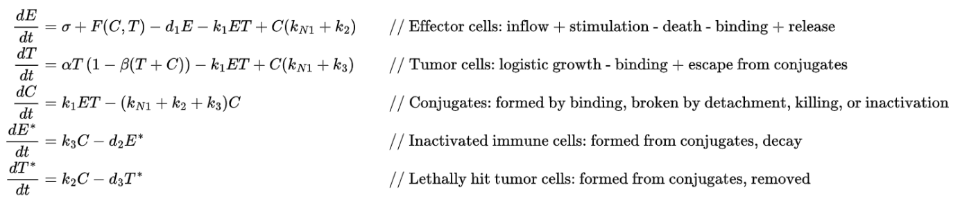
This mathematical model represents the effector cells response to the growth of an immunogenic tumor. This model differs from most others
in the literature in that it takes into account the infiltration of the tumor by eTLs as well as the possible effects of effector cell inactivation, seen by E* and T*.

Defining Parameters

Before we can explore the model, we first have to set the parameters. A large majority of the parameters were from Kuznetsov et al.’s paper with the rest being set based on norms in tumor biology.

◼

σ - 13000, Constant source rate of effector immune cells (per unit time)

In[]:=

σ=13000;

◼

d1 - 0.0412, Natural death rate of effector cells

In[]:=

d1=0.0412;

◼

η - 2.019×10^7, Saturation constant in stimulation function

In[]:=

η=2.019*10^7;

◼

ρ - 0.1245, Immune stimulation rate

In[]:=

ρ=0.1245;

◼

Fc[C,T] - (ρ*C[t])/(η + T[t]), Immune recruitment due to conjugate and tumor presence

In[]:=

Fc[C_,T_]:=(ρ*C)/(η+T)

Inactivated Immune and Lethally Hit Tumor Cell Removal:

◼

d2 - 0.05, Death rate of inactivated immune cells

In[]:=

d2=0.05;

◼

d3 - 0.00075, Removal rate of lethally hit tumor cells

In[]:=

d3=0.00075;

Tumor Growth Parameters:

◼

α - 0.1, Tumor growth rate

In[]:=

α=0.1;

◼

β - 2×10^−9, Inverse of tumor carrying capacity

In[]:=

β=2*10^-9;

Conjugate Dynamics:

◼

kN1 - 1, Detachment rate from conjugate

In[]:=

kN1=1;

◼

k1 - 1×^−6, Binding rate: E + T → C

In[]:=

k1=1*^-6;

◼

k2 - 1×^−2, Killing rate of tumor cells in conjugates

In[]:=

k2=1*^-2;

◼

k3 - 1.1×10^−6, Inactivation rate of effector cells in conjugates

In[]:=

k3=1.1*^-6;

After setting the parameters, we then plot the differential equations using Mathematica’s built-in NDSolve:

In[]:=

diffEquations=NDSolve[listEq,{e,T,c,EStar,TStar},{t,0,100},MaxSteps->∞];PlotEvaluate[ReplaceAll[{e[t],T[t],c[t],EStar[t],TStar[t]},diffEquations]],{t,0,100},



Out[]=

	Effector (e)
	Tumor (T)
	Conjugates (c)
	Inactive Immune (EStar)
	Dead Tumor (TStar)

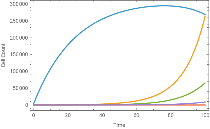
We can understand tumor-immune depending on the starting parameters, we can model the immune system fighting the tumor cells in different ways.

By changing the following parameters, the plot goes from the immune system failing to the immune system succeeding to kill the tumor cells:

In[]:=

α=0.8;d3=0.075;kN1=5;k2=0.75;

Sensitivity Analysis

Sensitivity analysis of our model is necessary in order to further understand which parameters impact which cells in a simpler manner. This sensitivity analysis algorithm will be used throughout this essay for the major models introduced.

Define sensitivityCalc to run model with parameter variations:

sensitivityCalc[{σ_,d1_,α_,β_,d2_,d3_,kN1_,k1_,k2_,k3_}]:={e'[t]==σ+Fc[c[t],T[t]]-d1*e[t]-k1*e[t]*T[t]+c[t]*(kN1+k2),T'[t]==α*T[t]*(1-β*(T[t]+c[t]))-k1*e[t]*T[t]+(kN1+k3)*c[t],c'[t]==k1*e[t]*T[t]-(kN1+k2+k3)*c[t],EStar'[t]==k3*c[t]-d2*EStar[t],TStar'[t]==k2*c[t]-d3*TStar[t],e[0]==3.3*^3,T[0]==10^2,c[0]==0,EStar[0]==0,TStar[0]==0};

Initialization of variables working to manipulate the parameters:

In[]:=

paras={{σ,0,0,0,0},{d1,0,0,0,0},{α,0,0,0,0},{β,0,0,0,0},{d2,0,0,0,0},{d3,0,0,0,0},{kN1,0,0,0,0},{k1,0,0,0,0},{k2,0,0,0,0},{k3,0,0,0,0}};constParaList={σ,d1,α,β,d2,d3,kN1,k1,k2,k3};labels={"σ","d1","α","β","d2","d3","kN1","k1","k2","k3"};

The iteration module going through and manipulating the necessary parameters:

In[]:=

Module[{senFunc,senAssoc,tumor,paraList={σ,d1,α,β,d2,d3,kN1,k1,k2,k3}},paras=Table[paraList[[i]]=paraList[[i]]*0.6;tumor=NDSolve[sensitivityCalc[paraList],{e,T,c,EStar,TStar},{t,0,100},MaxSteps->10^6];senAssoc=Association[tumor[[1]]];senFunc=Extract[senAssoc,{Key[e]}];lowVal=senFunc[99];lowFunc=senFunc;paraList[[i]]=constParaList[[i]]*1.4;tumor=NDSolve[sensitivityCalc[paraList],{e,T,c,EStar,TStar},{t,0,100},MaxSteps->10^6];senAssoc=Association[tumor[[1]]];senFunc=Extract[senAssoc,{Key[e]}];highFunc=senFunc;highVal=senFunc[99];paraList[[i]]=constParaList[[i]];{constParaList[[i]],lowVal,highVal,lowFunc,highFunc},{i,Length[constParaList]}];]

This module is fundamental to our sensitivity analysis. It first solves the system numerically for the perturbed parameter set through NDSolve, converts the solution into an association for easy access and extract the desired cell function (effector, tumor, conjugate, etc.), and stores the value of the desired cell function at the end of the time series after negative perturbation into the parameter record. The desired function is extracted with the function Key, with the function name being the parameter in this case being effector (e). Then, we do the same with the positive perturbation.

We then calculate the sensitivity index and plot it.

Create plot for the desired cell function (effector, tumor, etc.) with standard parameters:

Display plots for each parameter’s shift in a grid:

Calculate sensitivity index for each parameter and graph the values:

Through this graph, the left side is cell count after decreasing parameters by 40%, and the right is increasing parameters by 40%.
We can see that effector cells increase if σ, k1, or k2 increases or if d1, α, kN1 decreases (refer above to variable definitions). β, d2, d3, and k3 seem to have no impact on effector cell count. We can run this algorithm for the other 4 functions by changing the parameter in Key to understand relationships between parameters and functions further.

Simplified Tumor-Effector Model

Rihan et al. (2014) describes how if we assume that dc(t)/dt = 0, therefore c(t) = Ke(t)T(t) where K=k1/(kN1 + k2 + k3), Kuznetsov et al.’s model can be reduced to two equations which describe the behavior of effector and tumor cells only. We also incorporate a discrete time-delay 𝜏 into the model, which represents the delay by the immune system to respond to tumor cells after recognizing them. The behavior between these effector cells and tumour cells can reduce the size of both populations with different rates and parameters. We reuse many Kuznetsov et al. parameters, but get some more from Rihan et al. to set up this simplified model.

Overview of Rihan et al.’s simplified tumor-effector model -

As stated above, this model only focuses on tumor and effector cells. This interaction between the cells in the model expressed as −μA(t)B(t) and −nA(t)B(t) in dA/dt and dB/dt respectively. Rihan et al. also proves this model’s nonnegativity and boundedness solutions, allowing for the addition of treatment into this model. We then have to define our parameters for this new model.

Since the various models in this essay use the same symbols, we use Remove function as seen below to organize different models and ensure accuracy of the output.

Effector Immune Cell Parameters:

◼

μ – 3.422×10⁻¹⁰, Tumor-induced suppression rate of effector cells

◼

δ – 0.0412, Natural death rate of effector cells

◼

Old: σ, ρ, η

Tumor Growth Parameters

◼

r2 – 0.18, Intrinsic growth rate of tumor cells

◼

Old: β

Tumor–Immune Interaction Parameters

◼

n – 1.101×10⁻⁷, Rate at which effector cells kill tumor cells

◼

τ – 10, Time delay (days) for immune response to tumor changes

Initial Conditions

◼

A0 – 10⁶, Initial tumor cell population before t = 0

◼

B0 – 10⁶, Initial effector cell population before t = 0

Build the model with differential equations using NDSOLVE and plot the effector and tumor cells:

This model helps us to understand the oscillatory relationship between tumor cells and immune effector cells, highlighting how immune responses can temporarily suppress tumor growth, but may fail to eliminate it entirely. This leads to recurring tumor waves where the tumor is never killed but still decreases in size at some points of the graph, as seen in the oscillation dynamic of the system. This can reflect some cancers where tumors persist even with large effector populations attempting to block them or scenarios where the immune system gets exhausted. The model highlights the challenge the immune system faces when dealing with resilient tumors and emphasizes that only the immune system fighting tumors will not work for a complete extinction of the tumor cells.

Before extending the model to include chemotherapy, it is important to clarify the mathematical rationale for treating drug–tumor interactions as nonlinear amplification processes. Dr. Gabe Kwong’s work on activity-based cancer biomarkers introduced a multicompartment framework that interprets biological responses as catalytic, signal-amplifying systems rather than simple proportional reactions. His paper, “Mathematical framework for activity-based cancer biomarkers,” influenced how I constructed my chemotherapy terms, particularly the use of saturating, exponential, and amplification-driven dynamics to reflect realistic drug–tumor interactions. This mathematical perspective helped justify the shift from classical immune–tumor equations to a chemotherapy-augmented system that captures signal amplification and nonlinear therapeutic effects.

Chemotherapy Implementation into the DDEs

Explanation of Chemotherapy

Effector Cell Parameters

◼

ρ – 0.1, Maximum immune recruitment rate

◼

σ - 0.05, Constant source rate of effector cells

◼

τ – 1, Delay in immune system response

◼

δ – 0.2, Natural death rate of effector cells

◼

η – 0.3, Saturation constant in immune recruitment

◼

μ – 3.611×10 ⁻³, Inactivation rate of effector cells by tumor cells

◼

a1 – 0.2, Chemotherapy toxicity to effector cells

Tumor Cell Parameters

◼

r2 – 2.03, Growth rate of tumor cells

◼

β – 3×10⁻³, Inverse carrying capacity of tumor cells

◼

n – 1, Killing efficiency of effector cells on tumor cells

◼

c1 – 3×10 ⁻⁵, Inhibition rate of tumor cells by normal cells

◼

a2 – 0.4, Chemotherapy toxicity to tumor cells

Normal Cell Parameters

◼

r3 – 1, Growth rate of normal cells

◼

β2 – 10⁻³, Inverse carrying capacity of normal cells

◼

c2 - 3×10 ⁻⁹, Inhibition rate of normal cells by tumor cells

◼

a3 – 0.1, Chemotherapy toxicity to normal cells

Chemotherapy Parameters

◼

d1 – 0.01, Decay rate of chemotherapy drug in body

◼

d(t) – sqrt[t], Chemotherapy injection rate

Build the differential equation model:

Plot all 4 items:

Plot the functions logarithmically to analyze their dynamics more closely:

While we can see chemotherapy steadily increasing, it cannot completely eliminate the tumor. The immune system remains silent throughout the simulation, with effector cells showing minimal activation or expansion because of the presence of both tumor and chemotherapy which harms effectors throughout the model. After the tumor stabilizes, normal cells recover and dominate the system, indicating that chemotherapy does not have a large impact on normal cells in this setup. From a biological standpoint, the model reflects a scenario where chemotherapy slows tumor progression but fails to completely wipe it out. An explanation for this may be because of an absence of resistance in the model, which could highlight tumor evolution under treatment.

Chemotherapy Resistance:

To address the limitation of the current model, we introduce a chemotherapy resistance component into the model system, which is not implemented in any other DDEs including with Rihan et al.’s model. In this extended model, proposed exclusively in this essay, the total tumor population is divided into two subpopulations: chemo-sensitive tumor cells and chemo-resistant tumor cells. While the sensitive cells are affected by chemotherapy, a fraction of them convert into resistant cells over time due to continued drug exposure. These resistant cells are dramatically less responsive to chemotherapy, allowing them to persist and potentially dominate the tumor population. This addition allows the model to capture an important phenomenon observed in cancer therapy, where treatment initially appears effective but ultimately fails due to the emergence of drug-resistant tumor clones. In this section, we can explore how different treatment strategies influence tumor composition and the long-term success or failure of therapy.

Introducing the Equations and Assumptions

The first equation governs the dynamics of effector immune cells, V(t), incorporating delayed immune stimulation through tumor recognition (τ), activation via a saturating recruitment term, and depletion through tumor engagement, natural decay, and chemotherapy-induced cytotoxicity. The second and third equations describe the growth and suppression of sensitive tumor cells, Ts(t), and resistant tumor cells, Res(t), respectively. Both tumor populations grow logistically but are regulated by immune attacks, suppression from normal cells, and damage from chemotherapy. Notably, sensitive cells are more heavily affected by chemotherapy through direct killing and conversion into resistant phenotypes, while resistant cells persist under therapy but also experience some delayed drug impact.
The fourth equation tracks the dynamics of normal (healthy) cells, R(t), which follow logistic growth but are negatively affected by the tumor population and chemotherapy exposure. The final equation represents the pharmacokinetics of the chemotherapy drug concentration, u(t), with d(t) as the dosing input and d1 controlling decay or clearance of the drug. Initial conditions specify a starting population of immune cells, tumor cells (both sensitive and resistant), and normal tissue, with no drug present before treatment.

While containing many parameters, the model has some assumptions to simplify its mathematical analysis.

The model assumes that effector cells encounter and eliminate tumor cells proportionally to their quantity. However, in practice, this process is more complex, involving spatial constraints, signaling thresholds, and immune evasion tactics by tumors.

The model simplifies the emergence of drug resistance. Resistance is modeled as coming directly from sensitive cells under chemotherapy pressure, with logistic growth and natural selection competition between resistant vs. sensitive. While this captures a general trend, real-life resistance mechanisms involve genetic mutations, genetic reprogramming, and environmental shielding, which are not expressed in this model.

The model states sensitive and resistant cell types compete using a single logistic constraint (1−β(Ts +Res)). This assumes that both cells share the same resources and space, whereas real resistant cells might occupy different niches or retain alternative pathways.

After exploring the assumptions of the model, we can define the parameters. A majority of these parameters were self-defined based on norms throughout cancer patients and general biology.

Effector Cell Parameters

◼

ρ–0.33, Maximum immune recruitment rate

◼

σ–0.1, Constant source rate of effector cells

◼

τ–1, Delay in immune system response

◼

δ–0.21, Natural death rate of effector cells

◼

η–0.3, Saturation constant in immune recruitment

◼

μ–0.003611, Inactivation rate of effector cells by tumor cells

◼

ω–21, Natural growth rate of effector cells

Growth Parameters

◼

r1–1.03, Growth rate of sensitive tumor cells

◼

r2–1.5, Growth rate of resistant tumor cells

◼

r3–1, Growth rate of normal cells

Carrying capacity parameters

◼

β–2×10 ⁻³, Inverse carrying capacity of tumor cells

◼

β2–2×10 ⁻³, Inverse carrying capacity of normal cells

Interaction parameters

◼

n1–1, Killing efficiency of effector cells on sensitive tumor cells

◼

n2–0.01, Killing efficiency of effector cells on resistant tumor cells

◼

c1–3×10 ⁻⁵, Inhibition rate of tumor cells by normal cells

◼

c2–3×10 ⁻², Inhibition rate of normal cells by tumor cells

◼

c3–100, Fast growth feedback in sensitive tumor cells

Chemotherapy parameters

◼

a1–0.2, Chemotherapy toxicity to effector cells

◼

a2–0.4, Chemotherapy toxicity to sensitive tumor cells

◼

a3–0.05, Chemotherapy toxicity to resistant tumor cells

◼

a4–0.1, Chemotherapy toxicity to normal cells

◼

d1–0.01, Decay rate of chemotherapy drug in body

◼

d[t], Dosing function of chemotherapy, determines how much and often the chemo drug is administered

Drug resistance parameters

◼

b1–0.1, Induction rate: fraction of sensitive cells converted to resistant under chemo drug

◼

b2–14, Shift rate of sensitive to resistant under chemo exposure

◼

f1–0.3, Survival fraction of sensitive tumor cells after treatment

◼

f2–0.8, Survival fraction of resistant tumor cells after treatment

◼

time–100, Total simulation duration (in model time units)

Define chemotherapy resistance differential model and solve it:

Plot the time evolution of all populations:

In the model, we multiply chemotherapy by 100 for its visualization, as the units for chemotherapy throughout this model are count⁻². So to see the doses of chemo more clearly, we multiply it by 100. To analyze the model further, let’s plot other relationships. Let’s first make it easier to total tumor counts.

Define total tumor burden as functions:

Plot of tumor composition over time:

Plot tumor resistance ratio over time:

Log-scale plot for better visualization:

Plot 3-D phase space:

In order to ensure the model has biological significance, it is necessary to evaluate some theorems with this model.

The model satisfies the positivity of solutions, which states that all functions remain non-negative for all time and cell counts are not negative. Given that the system is composed of nonlinear growth, decay, and saturating terms, the structure of the equations prevents any variable from crossing below zero, provided the initial conditions are non-negative. We can also prove this by analyzing the plot.

In addition to positivity, the model satisfies boundedness, meaning that none of the populations can grow without limit over time, proven with the inclusion of carrying capacity parameters. Tumor and normal cells are governed by logistic growth with carrying capacities.

The model also satisfies a tumor-free equilibrium when a group of parameters differs slightly from the default, in which both sensitive and resistant tumor populations are reduced to near zero. This equilibrium reflects a scenario in which the immune system and chemotherapy are sufficient to eliminate the tumor, and normal and immune cells are at healthy levels.

Based on the 5 plots, we can present some takeaways:

◼

Tumor relapse is driven by resistant subclones that emerge under continuous chemotherapy pressure

◼

Single-mode therapy is insufficient because while chemo effectively killed sensitive cells, resistant cells survived and grew.

◼

The immune system is most active before resistance rises, so combining immunotherapy during that window could enhance treatment instead of later

◼

Therapy optimization could aim to suppress resistance emergence, possibly through adaptive chemo that is not redundant

◼

The immune system alone couldn’t control resistance, highlighting the need for chemotherapy or other treatments

Looking at the last takeaway specifically, we can prove this further by removing chemotherapy from the model and looking at the results.

Define differential model without chemo and solve it:

Plot the time evolution of all populations:

Plot of tumor composition over time:

Plot tumor resistance ratio over time:

Plot 3-D phase space:

These plots highlight how tumors can self-sustain and evolve, evolution can produce resistant clones in addition to chemotherapy, and that the immune system alone without additional help cannot stop tumor growth. The key concepts seen in the plots are unchecked tumor progression and natural resistance development to chemotherapy.

Chemotherapy Treatment Optimization and Analysis

To fully understand this cancer treatment model, a deeper analysis is required that extends beyond basic model simulation. By doing this, it allows us to make clinically actionable insights for cancer therapy decisions through the evaluation of the methods described in this section, like parameter sensitivity, uncertainty quantification, treatment optimization, and biomarker validation.

Redefine variables to avoid overlapping definitions:

Parameter Sensitivity Analysis

To begin our computational analysis, we can run a sensitivity analysis. Since the main goal of cancer treatment is killing tumor cells, we will start with our sensitivity analysis to just tumor growth/decay parameters and their individual impact on both sensitive and resistant tumor cells.

Define runModelWithParams to run model with tumor parameter variations (similar to sensitivityCalc function aforementioned):

Create the sensitivity analysis through iteration:

Display the sensitivity analysis plots:

A key reason why a shift in r1 and a2 (growth rate of, and chemotherapy’s toxicity to, sensitive tumor cells, respectively) does not affect tumor burden significantly is because at t=10 where the total is calculated, sensitive tumor cells are already at a extremely minimal value as compared to resistant tumors. This causes shifts to sensitive tumor cells to be almost negligible.

We can prove this by checking sensitive tumor’s quantity at t=10

Adaptive Dosing Strategy

Create adaptive dosing function and set adaptive parameters

Create and solve the model with near similar equations as previously with adaptive dosing added:

Plot the model with adaptive dosing:

When analyzing the plot, we can see the eradication of the tumor population with the growth of the immune cells. The adaptiveness of chemotherapy is seen with its decline after the tumor cells declined. With these details, it’s clear that the plot illustrates the effectiveness of an adaptive dosing strategy in controlling tumor growth while supporting immune recovery.

Treatment Comparison

We can confirm the effectiveness of adaptive chemotherapy by comparing the 3 types of chemotherapy dosing: continuous, intermittent, and adaptive.

Define treatmentComparison function to compare the different treatment protocols:

The function stores a different chemotherapy differential equation depending on the protocol of continuous, adaptive, or intermittent. Then, it solves the system of DDEs with each chemotherapy equation and plots the results.

Visualize the results of the function:

The results of this plot confirm the hypothesis that adaptive dosing of chemotherapy is the best for cancer treatment. While it may be plausible to characterize continuous dosing as the best dosing because the end tumor totals are similar, the fact that continuous dosing kills more immune cells, harming the body, along with tumor cells spiking significantly higher with continuous dosing, adaptive dosing seems to be the best for cancer treatment.

Multi-Objective Optimization

To further refine chemotherapy treatment strategies, we implement a multi-objective optimization for key therapeutic goals. Specifically, to minimize tumor burden, minimize drug-induced toxicity, and maximize immune response. The immune response is inversely related to tumor burden, reflecting that a lower tumor count has a immune presence. Toxicity is estimated based on chemotherapy parameters that contribute to side effects. Using a population of randomly generated treatment parameter sets, we apply Pareto frontier analysis to identify combinations that offer the best trade-offs. The resulting 3D plot highlights all candidate solutions and the Pareto-optimal subset, those not outperformed in all objectives simultaneously. This approach allows for treatment strategies that prioritize tumor control and overall patient well-being.

Define objective function: objectives - (minimize tumor, minimize toxicity, maximize immune response)

This function runs the tumor-immune-chemo model using the input parameters and calculates the tumor size, adds up toxicity which a2 and a3 parameters, and estimates immune strength as inversely related to tumor size. The desired outputs are as followed: smaller values are preferred for tumor and toxicity, and a larger (negative) value is preferred for immune response.

Pareto frontier analysis function:

The format of this function are as follows: generate random parameter sets close to the original values, evaluate the 3 objectives seen in the previous function, remove failed simulations, and then conduct the Pareto set analysis. This collects all optimal solutions into a list and plots them on a 3D grid.

This runs the Pareto analysis with 100 different trials to pick the parameter values with the most solutions:

From the plot, we can observe that most Pareto-optimal points lie along a region where tumor burden is relatively low, toxicity is moderate, and immune response is more favorable. This suggests that the optimal balance involves avoiding overly aggressive treatments that drive toxicity too high while still maintaining enough pressure on the tumor to reduce its size and preserve or stimulate immune response. The spread of the red points indicates the non-uniqueness of optimal solutions so that clinicians may prioritize different trade-offs depending on patient condition (like maybe minimizing toxicity in frail patients but trying to minimizing tumor in aggressive patients). Also, it proves the complexity of decision-making with treatment.

Stochastic Model

While differential models have been useful for understanding average tumor-immune-drug dynamics under ideal conditions, they fail to account for the randomness and variability through mutations, immune fluctuations, or irregular drug metabolism present in real biological systems. Therefore, incorporating a stochastic model allows us to simulate more realistic scenarios and assess treatment strategies under unpredictable conditions.

Building the stochastic model:

Perform Monte Carlo simulation by iterating the stochastic model multiple times to extract the final total tumor burden and compute statistical summaries like the mean, standard deviation, and a 95 % confidence interval:

Display the monte carlo results:

The distribution appears roughly symmetric and tightly clustered, indicating consistent outcomes under the given conditions. These statistics suggest that despite incorporating biological noise, the model outcomes are highly stable and predictable for this parameter set.

Biomarker Graphs

To enhance the interpretability of the tumor-immune-resistance model, we developed a comprehensive biomarker framework that tracks key biological metrics over time. This can help our model improve its communication ability and analyze important, yet simple metrics.

Here are the functions I use for my biomarker graphs:

◼

Total Tumor: Measures overall disease burden

◼

Resistance Fraction: Proportion of drug - resistant cells

◼

Immune Efficiency: Ratio of immune cells to tumor cells

◼

Tumor Burden: Logarithmic measure of tumor size

◼

Chemo Sensitivity: Weighted average drug sensitivity

◼

Tumor Heterogeneity: Measure of sensitive/resistant cell balance

◼

Tissue Health: Ratio of normal to total cells

◼

Treatment Response: Relative change in tumor burden

◼

Resistance Risk: Combined measure of resistance and tumor size

◼

Overall Survival Index: Composite measure of patient outcomes

Redefine the equations:

Primary biomarkers such as the ones below can capture essential mechanistic behaviors that are not always visible from state variables alone.

The total tumor (blue) initially lowers but then rises sharply after 𝑡≈60 shows eventual tumor escape. The resistance fraction (red) quickly reaches near 100%, showing that the tumor becomes entirely resistant early in treatment. The immune efficiency (green) peaks around 𝑡=10 but then rapidly declines to near zero. This graph indicates treatment failure due to the dominance of resistant tumor cells and the loss of immune control. The model suggests that although initial therapy may temporarily suppress the tumor, resistance rapidly takes over and immune support is insufficient to sustain long-term suppression, highlighting the need for both preventing resistance and sustaining immune activation.

We also define prognostic biomarkers which provide predictive insights into treatment durability and relapse risk:

In the plot, tumor heterogeneity (red) spikes early and then stabilizes at a low level, suggesting initial coexistence of sensitive and resistant cells followed by dominance of resistance. Immune exhaustion (orange) rises steadily and peaks sharply around t=60, coinciding with the tumor resurgence seen previously, before stabilizing highly. Meanwhile, tissue health (green) shows early recovery but collapses dramatically after t=60. These trends indicate a poor prognosis where the immune system becomes overwhelmed just as resistant tumor cells take over, leading to high exhaustion and diminished normal tissue function. The decline in tumor heterogeneity burden reinforces that resistant tumors dominate, while falling tissue health highlights the system’s failure to maintain balance and highlighting the need for earlier intervention.

To better inform clinical decisions, we introduce composite biomarkers which synthesize multiple variables into singular outcomes:

In this plot, treatment response (blue) peaks early but steadily declines to near zero, indicating poor long-term effectiveness, matching with previous assumptions of invalidity of continuous chemotherapy. Overall survival index (green) initially improves but drops sharply after t=60, aligning with tumor relapse and immune collapse. Meanwhile, resistance risk (red) rises gradually and plateaus at a high level, signaling persistent resistant tumor dominance. These results suggest that although treatment initially appears beneficial, its efficacy rapidly fades as resistance builds and survival outcomes worsen. The growing resistance risk and collapsing survival index reinforce the need for adaptive chemotherapy treatments.

We also implement a biomarker correlation matrix to identify relationships between features, highlighting predictors:

This biomarker correlation matrix shows several relationships. Immune efficiency is negatively correlated with total tumor, resistance fraction, and tumor burden, so when tumor growth and resistance increase, immune performance declines. In contrast, treatment response shows strong positive correlation with tissue health and immune efficiency, and strong negative correlation with tumor-associated metrics. This can highlight which biomarkers move together and which are inversely related, aiding in clinical interpretation and model validation. By identifying clusters of tightly correlated features, the matrix helps prioritize effective biomarkers for treatment monitoring and simplification of a composite index in predictive cancer decision-making.

For the alert system below, the graph shows how the tumor size and tumor resistance level change over time, along with red and orange lines that represent critical warning thresholds. When the tumor size or resistance line crosses these horizontal threshold lines, it means the cancer has grown too large or become too resistant, triggering a clinical alert that the treatment may no longer be effective.

We include clinical threshold alerts to further translate the model’s output into decisions by flagging key time points where tumor burden, resistance, or immune status exceed clinically meaningful limits:

Conclusion

In this study, we developed and analyzed a comprehensive tumor-immune-chemoresistance model incorporating chemotherapy, immune dynamics, and drug resistance mechanisms. By simulating treatment outcomes under adaptive and continuous dosing schedules, we demonstrated that adaptive dosing offers a more favorable balance between tumor suppression, immune preservation, and reduced toxicity. We further introduced a multi-objective optimization framework using Pareto front analysis to identify optimal treatment strategies that minimize tumor burden and toxicity while maximizing immune response.

To bridge model outputs with clinical relevance, we proposed a dynamic biomarker framework that captures key aspects of tumor progression, immune status, and treatment efficacy. Through primary, prognostic, and composite biomarkers, along with a correlation matrix and threshold-based alert system, we provided a data-driven foundation for medical decision support. Together, these tools enable deeper understanding of cancer dynamics and move personalized therapy design within cancer treatment forward.

This work highlights how mathematical modeling can capture the dynamic complexity of cancer progression and treatment resistance. We demonstrate how traditional treatments may inadvertently promote resistant tumors by extending normal tumor-immune models to include delay, chemotherapy, and resistance mechanisms. Biomarker correlations provide clinically relevant insights for evaluating therapy efficacy. Furthermore, multi-objective optimization reveals that adaptive chemotherapy regimens can have a better balance for reducing tumor size, preserving immune function, and limiting toxicity. These findings advocate for personalized, feedback-driven treatment plans and showcase the value of modeling in guiding future chemotherapy strategies.

Future Directions

Further work should focus on incorporating patient-specific clinical data into the model, allowing for individualized parameter estimation and treatment simulations with real-world cases. This can enable more personalized therapy optimization and more accurate biomarker interpretation. Additionally, incorporating spatial modeling for tumor microenvironment heterogeneity or agent-based simulations can further explore resistance evolution and immune-tumor interactions. Lastly, translating the biomarker and alert system into a clinical decision-support interface can enable direct application of model insights to oncological practice, helping clinicians make decisions about treatment in real time.

References

◼

Alfarouk, K. O., Stock, C.-M., Taylor, S., Walsh, M., Muddathir, A. K., Verduzco, D., Bashir, A. H. H., Mohammed, O. Y., Elhassan, G. O., Harguindey, S., Reshkin, S. J., Ibrahim, M. E., & Rauch, C. (2015). Resistance to cancer chemotherapy: failure in drug response from ADME to P-gp. Cancer Cell International, 15(1). https://doi.org/10.1186/s12935-015-0221-1

◼

Blais, J., & Jeukens, J. (2024). Pareto task inference analysis reveals cellular trade-offs in diffuse large B-Cell lymphoma transcriptomic data. Frontiers in Systems Biology, 4. https://doi.org/10.3389/fsysb.2024.1346076

◼

Davodabadi, F., Sajjadi, S. F., Sarhadi, M., Mirghasemi, S., Nadali Hezaveh, M., Khosravi, S., Kamali Andani, M., Cordani, M., Basiri, M., & Ghavami, S. (2023). Cancer chemotherapy resistance: Mechanisms and recent breakthrough in targeted drug delivery. European Journal of Pharmacology, 958(10), 176013. https://doi.org/10.1016/j.ejphar.2023.176013

◼

Kuznetsov, V., Makalkin, I., Taylor, M., & Perelson, A. (1994). Nonlinear dynamics of immunogenic tumors: Parameter estimation and global bifurcation analysis. Bulletin of Mathematical Biology, 56(2), 295–321. https://doi.org/10.1016/s0092-8240(05)80260-5

◼

Kwong, G. A., Dudani, J. S., Carrodeguas, E., Mazumdar, E. V., Zekavat, S. M., & Bhatia, S. N. (2015). Mathematical framework for activity-based cancer biomarkers. Proceedings of the National Academy of Sciences, 112(41), 12627–12632. https://doi.org/10.1073/pnas.1506925112

◼

Luozhong, S., Liu, P., Li, R., Yuan, Z., Debley, E., Chen, Y., Hu, Y., Cao, Z., Cui, M., McIlhenny, K., McCurdy, C., Bhashyam, D., Wilkens, S., Zhang, P., Kwan, A., Grossman, M., Lai, R., Ma, Y., Lipkin, S., & Jiang, S. (2025). Poly(carboxybetaine) lipids enhance mRNA therapeutics efficacy and reduce their immunogenicity. Nature Materials, 24(11), 1852–1861. https://doi.org/10.1038/s41563-025-02240-8

◼

Mansoori, B., Mohammadi, A., Davudian, S., Shirjang, S., & Baradaran, B. (2017). The Different Mechanisms of Cancer Drug Resistance: a Brief Review. Advanced Pharmaceutical Bulletin, 7(3), 339–348. https://doi.org/10.15171/apb.2017.041

◼

Otunuga, O. (2025). Stochastic modeling and first-passage-time analysis of oncological time metrics with dynamic tumor barriers. Scientific Reports, 15(1). https://doi.org/10.1038/s41598-025-95475-z

◼

Rihan, F. A., Abdelrahman, D. H., Al-Maskari, F., Ibrahim, F., & Abdeen, M. A. (2014). Delay Differential Model for Tumour-Immune Response with Chemoimmunotherapy and Optimal Control. Computational and Mathematical Methods in Medicine, 2014, 1–15. https://doi.org/10.1155/2014/982978

◼

Zhou, Y., Tao, L., Qiu, J., Xu, J., Yang, X., Zhang, Y., Tian, X., Guan, X., Cen, X., & Zhao, Y. (2024). Tumor biomarkers for diagnosis, prognosis and targeted therapy. Signal Transduction and Targeted Therapy, 9(1), 1–86. https://doi.org/10.1038/s41392-024-01823-2

Acknowledgements

I would like to thank my mentor, Dr. David DeBrota, for his continued support and guidance throughout my project. My project explored areas of tumor biology that I had not explored before, and he was extremely helpful in teaching me these concepts so I complete my project. I would also like to thank Dr. Young of Rice University for introducing me to biotechnology and getting me interested in the subject. Special thanks to the TAs and the directors Rory, Megan, and Eryn for their leadership and encouragement.

CITE THIS NOTEBOOK

Modeling tumor-immune interactions with chemotherapy via delay differential equations
by Sarim Mominkhawaja
Wolfram Community, STAFF PICKS, July 10, 2025
https://community.wolfram.com/groups/-/m/t/3499338