Ceva’s trisectrix, also known as the Ceva cycloid, is a classical plane curve associated with the trisection of an angle. This notebook presents the geometric construction of the curve, derives its parametric and Cartesian equations, and illustrates the construction through two dynamic visualisations: a planar animation and a three-dimensional rotational extension. A final section offers a playful reinterpretation in which the same curve is traced by the centroid of a moving triangle.
In an extra section (item 6) the geometric idea of how to make the trisection of the angle is added.
In an extra section (item 6) the geometric idea of how to make the trisection of the angle is added.
1. Geometric Construction and Parametric Equations
1. Geometric Construction and Parametric Equations
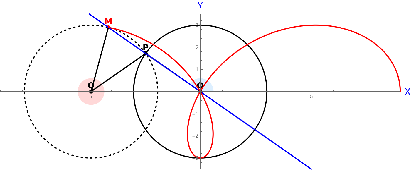
The Ceva trisectrix is generated by a simple geometric mechanism.
A point moves on a fixed circle of radius a centered at the origin . A second point lies on the x-axis and is chosen so that . The point is then defined as the intersection of the line with the moving circle of radius a centered at . As rotates around the origin, the locus of traces Ceva’s trisectrix.
P
Q
PQ = a
M
OP
Q
P
M
The construction is governed by the angle relation If we let then the geometry gives
∠XQM3∠XOP.
θ∠XOP,
◼
OP = PQ = QM = a
◼
∠XOP = ∠XQP
◼
∠XQM = 3θ
Hence the coordinates of are obtained as follows (see the 3. Animation 1: 2D Construction).
M
The x-coordinate is and the y-coordinate is Therefore, the parametric equations of the Ceva trisectrix are
xacos(θ)+acos(θ)+acos(3θ)a(cos(3θ)+2cos(θ)),
yasin(3θ).
M[θ_]:={a(Cos[3θ]+2Cos[θ]),aSin[3θ]};
2. Cartesian Equation
2. Cartesian Equation
Using the triple-angle identities we can rewrite the coordinates of as
cos(3θ)4(θ)-3cos(θ),
3
cos
sin(3θ)3sin(θ)-4(θ),
3
sin
M
M[θ_]:={a(4-Cos[θ]),a(3Sin[θ]-4)};
3
Cos[θ]
3
Sin[θ]
Eliminating θ from the parametric equations gives
Eliminate[{x==a(4-Cos[θ]),y==a(3Sin[θ]-4)},θ]//FullSimplify
3
Cos[θ]
3
Sin[θ]
From the factorized result, the defining factor of the Ceva trisectrix is
-+==0;
2
a
2
(-3+)
2
x
2
y
3
(+)
2
x
2
y
or, equivalently, .
3
+
2
x
2
y
2
a
2
3-
2
x
2
y
3. Animation 1: 2D Construction
3. Animation 1: 2D Construction
This animation displays the original planar mechanism and shows how the locus of is traced as the configuration evolves.
M
Manipulate[a=3;O1={0,0};P[θ_]:={aCos[θ],aSin[θ]};Q[θ_]:={2aCos[θ],0};M[θ_]:={a(Cos[3θ]+2Cos[θ]),aSin[3θ]};Show[{Graphics[{Black,PointSize[0.01],Point[P[t]],Text[Style["P",14,Bold],P[t],{0,-1.2}],{Red,Point[M[t]],Text[Style["M",14,Bold],M[t],{0,-1.2}]},Thick,Circle[O1,a],{Dashed,Circle[Q[t],a]},{LightBlue,Disk[O1,(a/5),{0,t}],LightRed,Disk[Q[t],(a/5),{0,3t}]},Line[{O1,P[t]}],Line[{P[t],Q[t]}],Line[{Q[t],M[t]}],{Blue,InfiniteLine[{O1,M[t]}]},Point[O1],Text[Style["O",14,Bold],O1,{0,-1.2}],Point[Q[t]],Text[Style["Q",14,Bold],Q[t],{0,-1.2}]}],ParametricPlot[M[θ],{θ,0,t},PlotStyle->{Red,Thick}]},AspectRatio->Automatic,Axes->True,AxesOrigin->{0,0},AxesLabel->(Style[#,15,Blue]&/@{"X","Y"}),PlotRange->{{-9,9},{-3.5,3.5}},ImageSize->700],Style["Trisectrix of Ceva",Bold,Large],{{t,0.32482,"Value (t)"},0.00001,2π,0.00001},SaveDefinitions->True,ControlPlacement->Top]
Out[]=


4. Animation 2: 3D Rotational Extension
4. Animation 2: 3D Rotational Extension
When the planar construction is rotated about the x-axis, it generates a three-dimensional surface. Visually, the resulting form resembles the atomic orbital , with two elongated lobes and a central equatorial ring.
d
2
z
If a planar curve in the xy-plane is written as then its rotation about the x-axis has the standard parametrization Applying this to the Ceva trisectrix gives
{f(θ),g(θ),0},
{f(θ),g(θ)cost,g(θ)sint}.
{a(cos(3θ)+2cos(θ)),asin(3θ)cost,asin(3θ)sint}.
a=3;O11={0,0,0};P1[θ_,t_]:={aCos[θ],aSin[θ]Cos[t],aSin[θ]Sin[t]};Q1[θ_]:={2aCos[θ],0,0};M1[θ_,t_]:={a(Cos[3θ]+2Cos[θ]),aSin[3θ]Cos[t],aSin[3θ]Sin[t]};Manipulate[Show[{ParametricPlot3D[M1[θ,t],{θ,0,t},PlotStyle->{Red,Thick}],RevolutionPlot3D[{a(Cos[3α]+2Cos[α]),aSin[3α],0},{α,0,π},{θ,0,t},RevolutionAxis->{1,0,0},PlotStyle->Opacity[0.6],Mesh->False,MaxRecursion->3,ColorFunction->"FruitPunchColors"],Graphics3D[{Black,Specularity[White,40],Ball[P1[t,t],0.15],Text[Style["P",14,Bold],P1[t,t],{1,-1}],{Red,Ball[M1[t,t],0.15],Text[Style["M",14,Bold],M1[t,t],{1,-1}]},Thick,Line[{O11,P1[t,t]}],Line[{P1[t,t],Q1[t]}],Line[{Q1[t],M1[t,t]}],{Blue,InfiniteLine[{O11,M1[t,t]}]},Ball[O11,0.15],Text[Style["O",14,Bold],O11,{1,-1}],Ball[Q1[t],0.15],Text[Style["Q",14,Bold],Q1[t],{1,-1}],Yellow,Opacity[0.1],Sphere[O11,a],Sphere[Q1[t],a]}]},BoxRatios->Automatic,Boxed->False,Axes->True,AxesOrigin->{0,0,0},AxesLabel->(Style[#,15,Blue]&/@{"X","Y","Z"}),PlotRange->{{-9,9},{-9,9},{-3.5,3.5}},ImageSize->700,ViewPoint->{1.3,-2.4,2.}],Style["Trisectrix of Ceva in 3D",Bold,Large],{{t,3.80748,"Value (t)"},0.00001,2π,0.00001},SaveDefinitions->True,ControlPlacement->Top]
Out[]=

5. A Geometric Game
5. A Geometric Game
The final section gives an alternative interpretation of the curve. Three points move on three circles and form a triangle. The challenge is to prescribe the motions so that the centroid of the triangle follows the parametric equations of the Ceva trisectrix.
The chosen positions of the circles are visually symmetric, but the underlying idea does not depend on this particular placement.
Manipulate[P1[t_]:={3Cos[t]-3,3Sin[t]+5};P2[t_]:={3Cos[t]-3,-3Sin[t]-5};P3[t_]:={3Cos[3t]+6,3Sin[3t]};tri={P1[t1],P2[t1],P3[t1]};M2[t1_]:=(P1[t1]+P2[t1]+P3[t1])/3;Show[{ParametricPlot[M2[t],{t,0,t1},PlotStyle->{Red,Thick}],Graphics[{{Blue,Thick,Circle[{-3,5},3],Circle[{-3,-5},3],Circle[{6,0},3]},Black,Thick,PointSize[0.01],Point[P1[t1]],Text[Style["P1",14,Bold],P1[t1],{0,-1.2}],Point[P2[t1]],Text[Style["P2",14,Bold],P2[t1],{0,-1.2}],Point[P3[t1]],Text[Style["P3",14,Bold],P3[t1],{0,-1.2}],{Red,Point[M2[t1]],Text[Style["M2",14,Bold],M2[t1],{0,-1.2}]},Line[{P1[t1],M2[t1]}],Line[{P2[t1],M2[t1]}],Line[{P3[t1],M2[t1]}],TriangleConstruct[tri,"Boundary"]}]},AspectRatio->Automatic,Axes->True,AxesOrigin->{0,0},AxesLabel->{x,y},PlotRange->{{-6,9},{-8,8}},ImageSize->700],{t1,3.41205,2π,0.00001}]
6. Geometric idea
6. Geometric idea
The procedure is as follows:
3. That line intersects the right lobe of Ceva's trisectrix.
4. The angle determined by the segment from the origin to that intersection point is the trisected angle.
7. Conclusions
7. Conclusions
◼
The animation clearly shows how a special curve, Ceva's trisectrix, can be used to construct the trisection of an angle.
◼
The method illustrates a fundamental distinction between what is impossible with straightedge and compass alone and what becomes possible when auxiliary curves are introduced.
◼
The quadrant adjustment is essential to maintain continuity and obtain the correct angular value over the full rotation.
◼
Wolfram Language provides an effective framework for combining visualization, symbolic computation, and interactive exploration in a single notebook.
8. References
8. References
3. AI
4. Personal notes