
This is the notebook which I have presented at 2023 Wolfram High School program on MultiParadigm Data Science for 2nd Level Certification.
In this work I describe, analyze and elaborate Central England Temperature historical time series, with data covering the years from about 1700 to 2019.
Some used methods are classical, other are innovative. In particular, a simple and intuitive algorithm for rank correlation between two temporal variables is formulated.
Also, some example of forecast is illustrated at the purpose of showing the power of forecasting tools offered by Mathematica.
Along this report-notebook, text explanations are inserted into cells having a light-brown background.
Notes or comments are inserted before the relative code instructions where considered necessary or useful.
All supplementary materials as data or references papers are collected as files in the same notebook directory.
Questions for the project
Questions for the project
This project would answer to the following questions:
◼
Can Temperature time series trend be explained by statistical autocorrelation or it should required some external agent? This question is important to verify if current increasing trend of (global, not only for England) Temperature is due to some temporal forcing independent from Temperature itself, and in this case to describe the forcing candidate.
◼
What are the statistical models or mathematical tools that better describe the Temperature data distribution along the years range considered? The answer will clarify if current models or algorithm can approximate both trend and other statistical properties of Temperature time series.
◼
Is it possible to formulate a simple tool for ranking correlation and causation among temporal variables other than Granger test? Usual statistical tests, in particular those for testing causation (also named causality), are not very easy or intuitive and their results often are questionable, therefore it could be useful to formulate a simpler tool which generate informations in a more clear manner.
◼
Can current Mathematica forecasting tools predict Temperature trend with results compatible with those offered by current scientific papers using more sophisticated and expensive methods? This question is important to verify the capability of Mathematica to forecast in a realistic manner and to be considered, even in the field of scientific research, reliable alternative to other more complex and more expensive tools.
Wrangling about data
Wrangling about data
The data have been downloaded from Wolfram Data Repository, December 2022, using Wolfram Language code ResourceObject[“Hadley Center Central England Temperature (HadCET) Dataset”]and then translated as Wolfram mx file. Data have been cleaned, curated, catalogued and maintained by the English Body National Climate Information Centre and hosted by Hadley Centre at UK Met Office (web page https://www.metoffice.gov.uk/hadobs/hadcet ) from historical archives and modern experimental database. Detailed informations about methods and techniques used for archive construction are available in reference
[1]
.In[]:=
(*Importfromthefilemx:themaindatastructureisthatofaWolframTimeSeries*)SetDirectory[NotebookDirectory[]];tsHadleyTemperatures=Import["TEMPERATURE HADLEY.mx"]
Out[]=
TimeSeries


In[]:=
(*structureofthedatasetdefinedbyTimeSeries*)Map[<|#->tsHadleyTemperatures[#]|>&,tsHadleyTemperatures["Properties"]]//Dataset
Out[]=

An important item about temporal data is checking their distribution over time and presence of missing data:
In[]:=
(*checkifdataareregularlyspacedintime*)RegularlySampledQ[tsHadleyTemperatures]
Out[]=
True
In[]:=
(*asfromdatasetstructure,thetimeserieshasonlyoneone-dimensionalPath*)tsHadleyTemperatures["ValueDimensions"]
Out[]=
1
In[]:=
(*therearenomissingdataintimeseries*)Cases[tsHadleyTemperatures["Path"],{t_,missingData_Missing}:>{DateObject[t],missingData}]
Out[]=
{}
In[]:=
(*beingdataregularlyspacedintime,fromthefirsttwoentrieswecandeducethattimestepfromonedatatothenextisequaltoonemonth*)Take[tsHadleyTemperatures["Dates"],2]
Out[]=
,
Exploring data
Exploring data
In this section we explore some features of the dataset.
In[]:=
(*somefirstfeaturesofthedataset*)lengthHadley=tsHadleyTemperatures["PathLength"];firstDateHadley=tsHadleyTemperatures["FirstDate"];lastDateHadley=tsHadleyTemperatures["LastDate"];
In[]:=
(*thetemporalrangecoveredbythedata*)Print["The first date: ",firstDateHadley]Print["The last date: ",lastDateHadley]
The first date:
The last date:
In[]:=
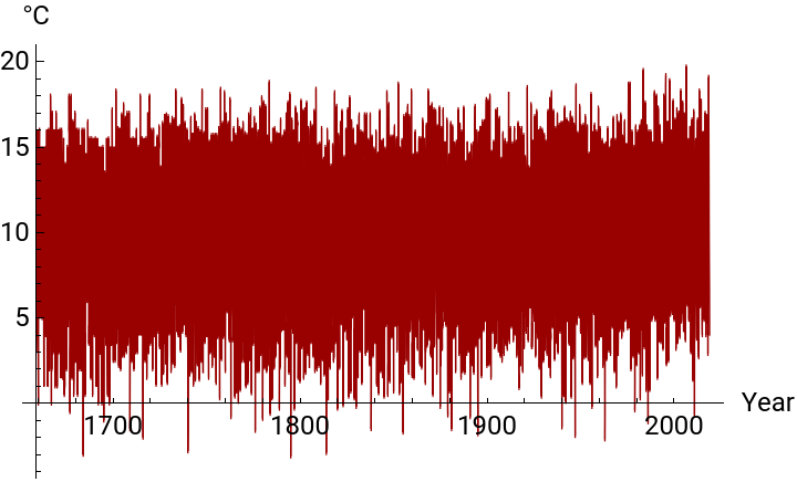
(*afirstvisualexplorationofTemperaturevalues*)(*note,fromdatasetstructure,thatthemeasureunitforTemperatureis°C*)DateListPlot[tsHadleyTemperatures,PlotStyleDirective[Thickness[0.002],RGBColor[0.6,0.,0.]],Frame->False,AxesLabel{"Year","°C"},AxesStyleDirective[Black,12],PlotLegends{"Monthly Temperature values"}]
Out[]=

The so-called Tukey’s Five Numbers Summary is a concise numerical representation of the main descriptive statistics about a set of data. All the five quantities are directly computed by Mathematica built-in functions.
In[]:=
(*TheTukey'sfivenumberssummary*)TextGrid[{{Style["The Tukey's five numbers summary",14,Bold]},{"Mean",meanHadley=Round[Mean[tsHadleyTemperatures],0.01]},{"Min",minHadley=Min[tsHadleyTemperatures]},{"Max",maxHadley=Max[tsHadleyTemperatures]},{"First Quartiles",firstQuartileHadley=First@Take[Quartiles[tsHadleyTemperatures],{1}]},{"Third Quartiles",thirdQuartileHadley=First@Take[Quartiles[tsHadleyTemperatures],{3}]}},Dividers->{False,Center}]
Out[]=
The Tukey's five numbers summary | |
Mean | |
Min | |
Max | |
First Quartiles | |
Third Quartiles |
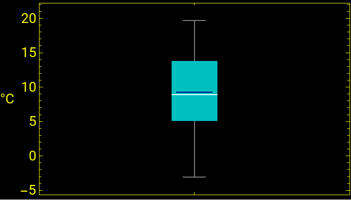
In the following visual representation, based on a Tukey box-plot graphics, it can be noted that First Quartile and Third Quartile are quite far respectively from the Min and the Max of the dataset values (move mouse over the cyan box), showing a large spread from Min to Max. The blu line in the Tukey rectangle identifies the Mean value, the white the Median.
In[]:=
BoxWhiskerChart[tsHadleyTemperatures,{{"MeanMarker",0.8,RGBColor[0.,0.,0.5]}},FrameLabel"°C",RotateLabelFalse,FrameStyleDirective[Yellow,14],ChartStyleRGBColor[0.,0.75,0.75],Background->Black]
Out[]=
The next graphics compares the Temperature values with their Mean and Standard Deviation: we can see that values (outliers) lower or upper than the Standard Deviation range [- Std Dev + Mean, Mean + Std Dev] are quite uniformly distributed along the years.
This is an Histogram of the Temperatures distribution, from which it is evident that the values do not follow a Normal Distribution centered on the Mean value, but they tend to accumulate on the low and high extremes of the Standard Deviation range. Also, the percentages of values lower and upper than these two extremes are computed: the two percentages are quite significative, showing that not only the numerical values, but even their distribution has a large spread.
Next graphics compares the trends of Temperature values, every 10 years, upper and lower than Standard Deviation range. Note that, while until 1900 the two trends are comparable, after 1900 they are well distinguishable: the amount of upper values tends to increase, that of lower tends to decrease: a first signal of the trend towards a warming environment.
Analyzing data
Analyzing data
In next section the data will be analyzed with some particular methods and algorithms for determining some key features and founding possible causes which could be the origin of that features.
As first operation, it is convenient (see e.g. [2]) to consider the new temporal data obtained subtracting the Mean value, so that to deal with a list of data having zero Mean. In the following of this report, expressions like “Deviations Temperature” will indicate this new and other analogous lists of data having zero Mean.
As first operation, it is convenient (see e.g. [2]) to consider the new temporal data obtained subtracting the Mean value, so that to deal with a list of data having zero Mean. In the following of this report, expressions like “Deviations Temperature” will indicate this new and other analogous lists of data having zero Mean.
Previous graphics is not easy to interpret: we try to have a more readable set of data gathering the mean values after partitioning data into consecutive subsets of fixed length equal to one year. In this way we construct a temporal data of the deviations, for each year, from Mean value.
Now temporal data are becoming more readable: as first qualitative result, note that starting from about 1950 the deviations are quite all positive, that is the Temperature values from the year 1950 are greater than the global Mean value computed in the entire temporal range 1659 - 2019. For a quantitative result, we evaluate the means every 10 years, using the Mathematica built-in function MovingAverage.
The trend of increasing Temperature values from about the middle of ‘900 years is more readable: a more clear graphics is the next plot where positive mean values and negative mean values are colorized by two different tones.
It is interesting to note that the very low mean Temperatures around the year 1700 are historically confirmed by the so-called “Little Ace Age” which has registered the colder values in the years 1709-1710 (see [3]), when in England the river Thames and in Italy the Venice lagoon were been frozen for many months.
From the two previous graphics, one can suspect the presence of some periodicity of values around the zero Mean until year 1900. For verifying this, we use a Fourier analysis by means of a Discrete Fourier Transform.
From the two previous graphics, one can suspect the presence of some periodicity of values around the zero Mean until year 1900. For verifying this, we use a Fourier analysis by means of a Discrete Fourier Transform.
The presence of periodicity in the data is tested by approximation using a Cosine Fourier expansions with a maximum order corresponding to the greater significative mode obtained from Fourier Transform. We define a procedure for the construction of this truncated trigonometric series; the frequency parameters used in this series must take into account all the parameters defined in the built-in function Fourier. The coefficients of the trigonometric polynomial are computed using a fitting by minimization of Least Squares residuals, as done by built-in FindFit function. Note that the approximation is very good, confirming the fact that original data have periodicities which convolve themselves.
Here we estimate the Accuracy of previous Fourier approximation, using the absolute value of the difference between a real value and the relative value computed with trigonometric polynomial. The accuracy so defined is very good in the range of years considered.
If the (deviations from global Mean) Temperature values would follow previous computed trigonometric polynomial approximation even after 1900, then forecasting until year 2000 using this approximation should give minimal residuals respect to experimental data. As shown by the following code and graphics, this is not the case.
The conclusion is that Temperature values after year 1900 do not follow the same periodic trend of the values from 1659 to 1900.
The conclusion is that Temperature values after year 1900 do not follow the same periodic trend of the values from 1659 to 1900.
As first attempt to search the reasons about the behavior of Temperature values in the 20th century, consider for example the first three significative modes of Fourier Transform (the mode 1 is not considered because it has zero frequency). These modes, marked as red in the graphics below, correspond to temporal periods which are, with good approximation, all multiple of the integer 11.
There is a natural, planetary (therefore not limited to Central England only) physical feature having a natural temporal period of about 11 years: the sunspots of our star, the Sun.
We consider the data about Solar TSI (Total Irradiation Index), which is a temporal series which values are the power per unit area received by the Earth from the Sun. The source is the archive [4] at NASA site. Data cover the range of years from 1610 to 2014.
We consider the data about Solar TSI (Total Irradiation Index), which is a temporal series which values are the power per unit area received by the Earth from the Sun. The source is the archive [4] at NASA site. Data cover the range of years from 1610 to 2014.
Here a first analysis of this temporal series.
Now consider the Fourier Discrete Transform of TSI data, as done for Temperature.
Note that, except the 2nd mode, the more significative peak is positioned near the 40th mode, exactly at mode 38, which corresponds to a temporal period of about 11 years, the period of sunspots.
And this is the construction of the Fourier trigonometric polynomial using these first four significative modes. The graphics below shows that these four modes are sufficient for a qualitative approximation of the main periodicities of the original data.
It is interesting to compare the temporal periodicity from Fourier analysis with the periodicity estimated by a statistical process approximating the TSI data. In next section, the best process is estimated using the SARMA Family models, which specific parameters are chosen on the basis of usual Information Criterions like Akaike AIC (see [2]). The seasonality computed by the best fitting process is 11 years, confirming the result from previous Fourier analysis.
Our aim is to compare Anthropogenic Forcing values (RFAnth) with Temperature Deviations from Mean along the 20th century.
The first step is to identify a convenient Fourier trigonometric polynomial for approximation of Temperature Deviations trend.
The first step is to identify a convenient Fourier trigonometric polynomial for approximation of Temperature Deviations trend.
For a better justification of this Fourier trigonometric approximation, we would compare it with trend estimated by the Hodrick-Prescott Filter, a popular tool in Data Analysis (see e.g. [2]). Using a function for computing a list of values by means of this algorithm, we can compare Fourier and HP Filter results: the plot below shows a substantial equivalence between the two methods.
Now we find a Fourier approximation to the Anthropogenic Forcing data, using the same maximum order as that already used for Temperature data. The aim is to discover a possible correlation between the two sets of data.
As we want to have a qualitative information, no matter if we compare different units of measure and different amounts between the two dataset.
We analyze the second Differences of data, that is the discrete Derivative of the first Discrete Derivative. This tool shows the changes in curvature of previous graphs and is important for finding correlation or causation among temporal variables (see [2]).
As first thing, a function is introduced for finding the zeros of the second Differences of data by means of a simple algorithm which checks the sign of the product of two temporal consecutive values of these 2nd differences: if the product is negative, there is a change of sign and therefore a zero between them. It is then simple compare the temporal 2nd differences series of (Fourier approximated) Temperature and Anthropogenic Forcing for finding qualitative informations about correlation or causation.
The 2nd differences of the two time series are computed using the built-in Wolfram function Differences.
Next two graphics illustrate previous numerical results: black and grey correspond to (2nd differences) Anthropogenic Forcing, red and light-red to Temperature. Note that “red” follow the trend of “black”, so that we can deduce that, at least qualitatively, Anthropogenic variable causes Temperature variable, that is starting from about the middle of 19th century the Temperature deviations from global Mean values are strongly influenced by emissions due to human activities.
Next graphic tool is also useful for qualitative analysis of correlation and causation: for the last three centuries, Anthropogenic and Temperature data are collected into histograms representing respectively the distributions of values and deviations from Mean (bin width = 0.5, the range [-2, 4] are negative or positive deviations jumps). The increasing distribution towards upper values for Anthropogenic variable (gray) drives an increasing distribution of Temperature deviations (red) towards values greater than Mean value (move the mouse over the histograms bars to visualize the amount of values falling in each bars).
For a quantitative approach to evaluate the correlation-causation of the two time series, the better tools are the statistical processes which can model the temporal data.
As first attempt, consider the VAR Process family, that is Vector Autoregression models. In a VAR Process, the values at time t of two or more temporal variables are dependent on their values registered on previous time steps t - 1, t - 2, ..., t - k, being k the order lag of the model (see [2], [7]; also, see [8] for application of VAR method on climatology). A VAR statistical process should be used for modeling a time series only if data are stationary (see [2]), that is if Mean and Standard Deviation are constant in time. In our case, from previous graphics Anthropogenic Forcing and Temperature have not constant Mean, but quantitative informations can be obtained with the following simple method which is based on fitting a VAR-like mathematical model to our data.
At first, we try to find the better order-lag to our mathematical model. Mathematica can estimate a VAR model using the built-in function EstimatedProcess and an assigned order. So, we define a function which accepts as input the vector data and the order, and returns as output the order, the parameters of the estimated VAR model and the value of the corresponding vectorial AIC Information Criterion. The result of this estimate is that the best model, up to order 5, belonging to the VAR Family is the model of order 1: VAR(1).
In all the next sections, the expression dataVectList will be the structure of data of the form {t, A [t], T[t]}, where A = Anthropogenic Forcing, T = Temperature experimental data.
Note that the so computed entries of the constant vector V and of the matrix M are close to those of the constant vector and Autoregression matrix of previous estimated VAR(1) model. We check that previous analytical model, based on order 1 VAR process, is a quite good approximation of the real data.
From the entries of the matrix M of the analytical model, it can be inferred that the dependence of A[ t ] on T[ t – 1 ] is very weak, while the dependence of T[ t ] on A[ t – 1 ] is significative.
Next two graphics give the more important qualitative information from our analysis.
In the first, experimental data (light red) of (Deviations from Mean) Temperature are compared with those estimated by (Equation 1) of previous analytical model (red), with those computed from previous equation for T[ t ] with M[2, 1] = 0 (Temperature-only estimation, gray), that is without the influence of Anthropogenic Forcing, and those computed for T[t] with M[2, 2] = 0 (RFAnth-only estimation, black), that is with the influence of only Anthropogenic Forcing. It is evident that the values T[ t ] computed only on previous values of only T variable don’t agree with the trend of experimental data. The conclusion is that , for our model, Temperature trend in the temporal range from 1850 to the first decade of 21st century is determined by the trend of Anthropogenic Forcing due to greenhouse emissions.
On the contrary, in the second graphics it is shown that the values of Anthropogenic Forcing computed with the model agree well with experimental data even without the contribution of Temperature.
The qualitative conclusion is that Anthropogenic Forcing due to greenhouse emissions causes Temperature, while vice versa is not true.
Note that this result agrees with [5], where an analogous conclusion is reached using methods based on neural networks.
Now we try to quantify previous qualitative results. A possible method could be to apply the Granger Causality Test (see [2]), but its numerical estimation of the amount of influence of one temporal variable on another is based on a quite abstruse algorithm. Here we propose a more simple but effective algorithm, which therefore could be considered a method for ranking both correlation and causation between two variables.
First, if P and Q are two temporal variables, compute the euclidean norm (Norm[V, 2]) PQ of the numerical list V obtained computing the difference of the Q[ t ] values estimated by model equations (Equation 1) and the Q[ t ] values estimated using only P[ t – 1 ] values. If P is not Q and P strictly causes Q, that is if P is essential for Q, than PQ is small compared to the other QP, PP and QQ values; if P is not Q and P does not cause Q, than PQ is great.
Then, compute the four quantities p = (M – s)/M, being s ∈ { PP, QP, PQ, QQ } and M = Max { PP, QP, PQ, QQ }. Note that 0 ≤ p ≤ 1 and, if P causes Q and not vice versa, than (M – PQ)/M is a value next to 1 and greater than (M – QP)/M, which is next to 0.
The values p are disposed in a matrix form graphics where the expression P → Q represents the value (M – PQ)/M, so that, with the help of grading colors and their legends, it is easy to deduce if P causes Q and the numerical amount of this causation.
In our context, A = Anthropogenic Forcing, T = Temperature. The numerical values of the matrix entries clearly show that A causes T and not vice versa.
Forecasting
Forecasting
We now discuss the usage of some tools of Mathematica package for forecasting. From a scientific point of view, forecast matter about Temperature is a very crucial item even for social and economic reasons.
Note that forecasting using the analytical model of (Equation 1) is easy but quite not realistic, because the two variables are monotonically increasing and stochastic noisy is absent, so forecasted values tend to become huge without the presence of braking effects.
See below what happens to Temperature for a 100-years forecast, starting from the last values of the variables computed by the model. An increasing of about 3°C - 4°C for the end of 21th century is generally considered too high in the most scientific works about this item.
See what happens also forecasting by means of previous VAR(1) model. The forecasted values for Temperature and Anthropogenic Forcing are computed by the built-in function TimeSeriesForecast using the VAR(1) model for an horizon of 100 years.
The red and blue forecasting curves in the two graphics below are inserted between the upper and lower bands of mean squared errors. The trends of the two curves seem to be strange but they are not surprising: in fact, from theory (see [2]) a 1-order AR or VAR model predicts that the forecasted values of a variable tend asymptotically to the Mean value of (the process relative to) previous time series values of that variable. Note that the two asymptotic forecasts tend to the Mean values of Temperature and Anthropogenic Forcing.
This first forecast method seems to be not satisfactory, because its predictions are not justified by all previous analysis.
Therefore we can deduce that a statical process model could be effective for approximating real measured data, but it could be not appropriate for forecasting purposes.
For a more realistic forecast, we should use a more complex statistical process: we try a Vector ARIMA (VARIMA), because for this type of process the long-term forecasts tend to be linear or more than linear, depending on the order of Integration parameters to be used, that is how many past time steps should be considered for estimate the current value of a variable (see [2]).
For simplicity, here we use 1-order Differences (green) for our two variables and 1-order for Auto-regression (red) and Moving Average (blue) process components: ARIMA(1, [1, 1], 1), which is performed by Mathematica expression ARIMAProcess[1, {1, 1}, 1] (see [9]).
The following instructions give the values of all the various components of the VARIMA model associated to the couple (Anthropogenic Forcing, Temperature).
Next graphics shows that the 1-order VARIMA model gives a satisfactory approximation for RFAnth and Temperature values.
The approximation is based on the relative time series of the annual mean values for a set of paths randomly computed using the estimated VARIMA process. The number of paths is choice to be 1000.
The approximation is based on the relative time series of the annual mean values for a set of paths randomly computed using the estimated VARIMA process. The number of paths is choice to be 1000.
Now we can forecasting, with the choice of 2100 as last year forecasted and the built-in function TimeSeriesForecast which can perform a direct forecast.
Note that this VARIMA forecast is completely different and seems more realistic than previous VAR one.
Also, we can deduce a first conclusion from a scientific point of view: without decreasing the current trend of Anthropogenic Forcing, the predictions show that until the end of the 21st century the mean Temperature could increase by about 1.5°C as compared to current values. This result, obtained using a simple low-order model, is very similar to those obtained in scientific papers using more forcing variables and more complex tools (see e.g. [10] and [11]).
For a more complete analysis of possible forecasts, consider the method which uses random simulations of the VARIMA process, and then computes their average.
At first we choice a fixed number of paths, then each path (t, { A[t], T[t] }) for t until year 2100 is computed by the built-in RandomFunction using previous estimated VARIMA model; at the end, the Mean time series of all the paths for variables A and T is computed.
At first we choice a fixed number of paths, then each path (t, { A[t], T[t] }) for t until year 2100 is computed by the built-in RandomFunction using previous estimated VARIMA model; at the end, the Mean time series of all the paths for variables A and T is computed.
Next graphics shows the distribution histogram of the Mean Temperature forecasts, obtained using a statistically great number (e.g. 1000, in this case) of runs and computing, by previous method, the average of 100 random paths for each run. The distribution of these 1000 Mean values (referred to the current reference Mean value = 0°C) shows a significative main concentration in the range [1.6°C, 2.4°C], which is in a satisfactory agreement with the value 1.5°C of the forecast based on previous direct application of theoretical VARIMA model.
Conclusions
Conclusions
We can now answer to initial questions formulated for this project.
◼
Can Temperature time series trend be explained by statistical autocorrelation or it should required some external agent? The Temperature time series trend is weakly autocorrelated and it could be statistically explained by the Forcing variable due to anthropogenic greenhouse emissions.
◼
What are the statistical models or mathematical tools that better describe the Temperature data distribution along the years range considered? Trend and other properties, like presence of periodicity, for Temperature time series could be described with good qualitative and quantitative results using statistical models like those of Vector ARIMA processes and by Fourier Analysis approximations.
◼
Is it possible to formulate a simple tool for ranking correlation and causation among temporal variables other than Granger test? A mathematical ranking tool, simple to compute and easy to understand and to graphically visualized, has been formulated for finding numerical amount of correlation and causation between two temporal variables.
◼
Can current Mathematica forecasting tools predict Temperature trend with results compatible with those offered by scientific papers using more sophisticated and expensive methods? Current Mathematica built-in tools for forecasting can be used with good results as compared to other more sophisticated and computationally expensive methods which often are used in many scientific research areas.
Keywords
Keywords
◼
Time Series
◼
Fourier Transform
◼
Fourier Approximation
◼
Vector Autoregression for multivariate Time Series
◼
Rank correlation - causation algorithm
◼
Forecasting multivariate Time Series
References
References
[1] D.E. Parker, T.P. Legg and C.K. Folland, A new daily Central England Temperature Series 1772-1991, Int. J. Clim., 12, pp 317-342, 1992
[2] T . C . Mills, Applied Time Series Analysis, Academic Press, 2019
[3] E . Hawkins, G . Jones, M . Lockwood, M . Owens, I . Usoskin, Frost fairs, sunspots and the Little Ace Age, A & G, 58, Royal Astronomical Society, aandg . org, 2017
[4] https://data.giss.nasa.gov/modelforce/solar.irradiance/solar.lean2015.ann1610-2014.txt (page visited in December 2022)
[5] A. Pasini, P. Racca, S. Amendola, G. Cartocci, C. Cassardo, Attribution of recent temperature behaviour reassessed by a neural-network method, Nature Scientific Report, 7, 17681, 2017
[7] Wolfram Research, ARProcess, Wolfram Language function, https://reference.wolfram.com/language/ref/ARProcess.html
[8] W. Abdallah et al., A vector autoregressive methodology for short‑term weather forecasting : tests for Lebanon, Nature SN Applied Sciences, 2, 1555, 2020
[9] Wolfram Research, ARIMAProcess, Wolfram Language function, https://reference.wolfram.com/language/ref/ARProcess.html
[10] M. Mudelsee, Trend analysis of climate time series: A review of methods, Earth-Science Reviews 190, 310-322, 2019
[11] J. Contzen et al., Long-term temporal evolution of extreme temperature in a warming Earth, PLoS ONE 18(2), 2023
CITE THIS NOTEBOOK
CITE THIS NOTEBOOK
Modeling and forecasting historical time series of Central England temperature
by Gianluca Argentini
Wolfram Community, STAFF PICKS, June 5, 2024
https://community.wolfram.com/groups/-/m/t/3188208
by Gianluca Argentini
Wolfram Community, STAFF PICKS, June 5, 2024
https://community.wolfram.com/groups/-/m/t/3188208