Notebook by:
- Erin Dante de Oliveira Vasconcelos
- Lucas André Martins Queiroz
- Thiago Augusto Soares Souza
Supervisor:
- Prof . Rubelmar Maia de Azevedo Cruz Neto
- Erin Dante de Oliveira Vasconcelos
- Lucas André Martins Queiroz
- Thiago Augusto Soares Souza
Supervisor:
- Prof . Rubelmar Maia de Azevedo Cruz Neto
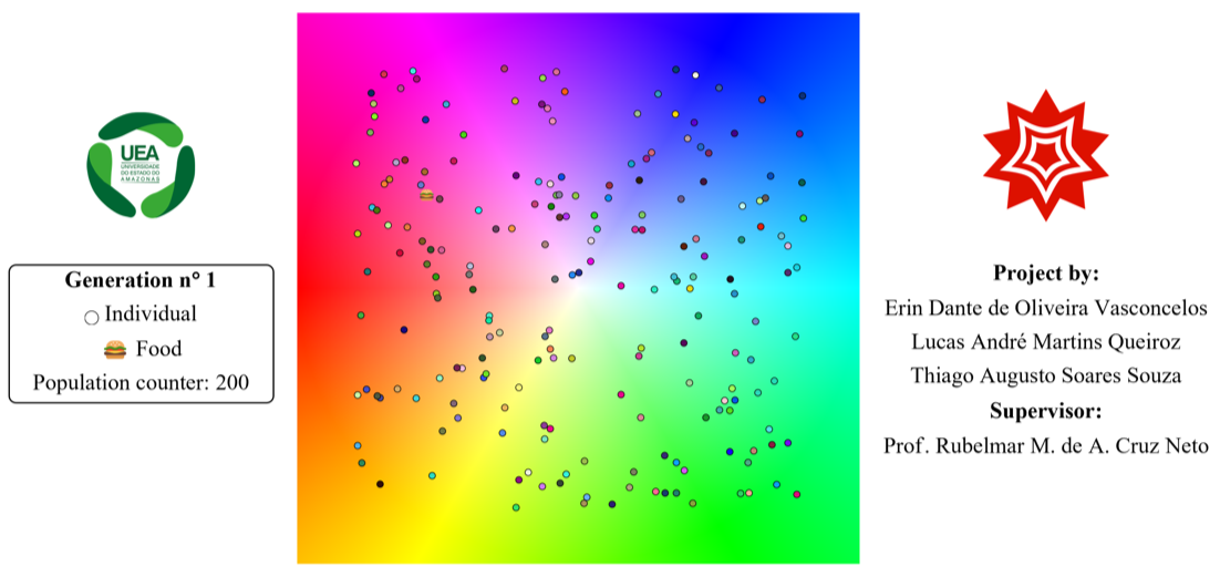
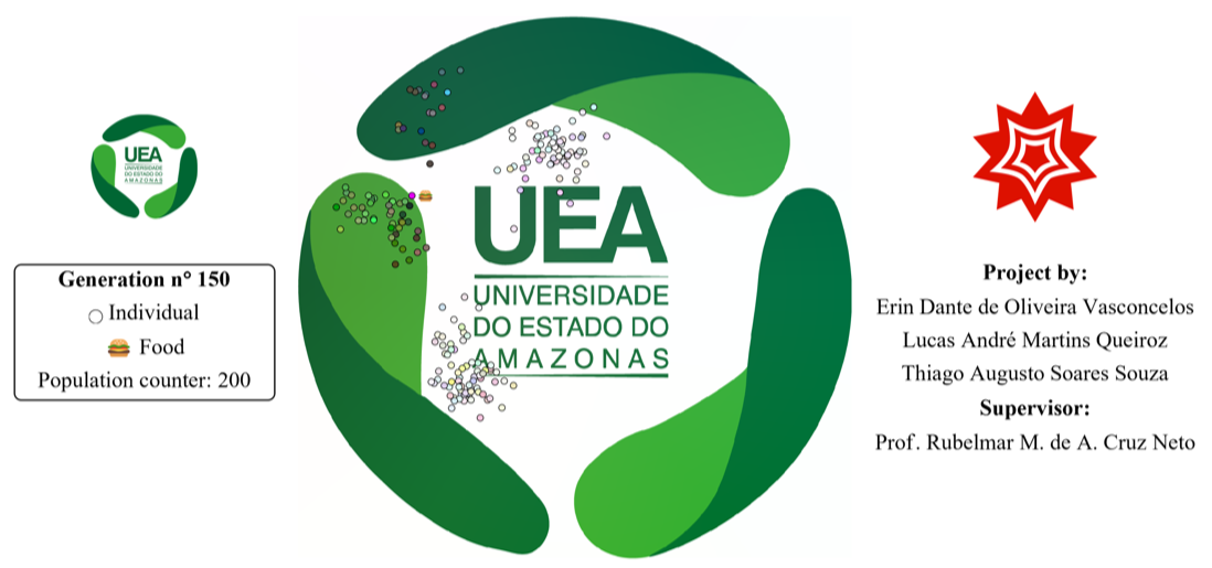
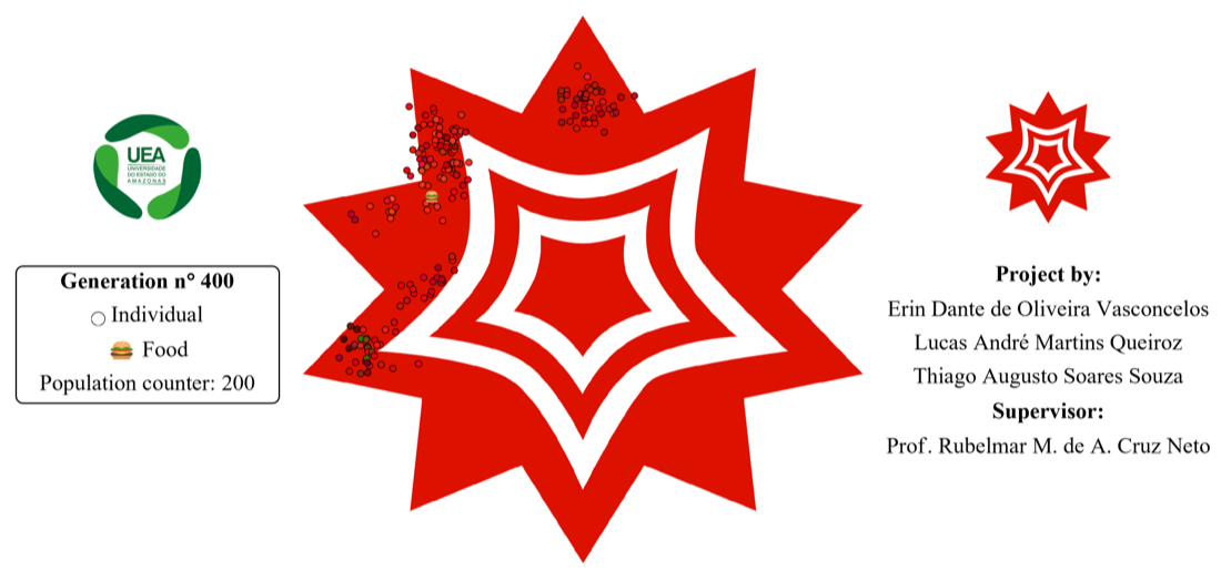
The algorithm simulates natural evolution and speciation by applying a mortality chance if the individual’s color is different from the background color and reducing this chance if it’s close to food.
Each individual only survives a few iterations, can only reproduce with nearby neighbors and the background slowly changes between iterations.
This project was inspired by Universo Programados’s video “Simulando a Teoria da Evolução!” on Youtube, available at: https://youtu.be/VqAuFnpF1TY
Each individual only survives a few iterations, can only reproduce with nearby neighbors and the background slowly changes between iterations.
This project was inspired by Universo Programados’s video “Simulando a Teoria da Evolução!” on Youtube, available at: https://youtu.be/VqAuFnpF1TY
Snapshots
Snapshots
Here some snapshots for a run of the algorithm.
Background
Background
The color square background was created on Mathematica and exported as PNG. The simulation backgrounds were generated first for better speed and memory usage.
In[]:=
colorSquare=Image@Table Module{r=Sqrt[x^2+y^2],θ,rgb,a}, θ=If[x==0&&y==0,0,ArcTan[x,y]+π]; rgb=ColorConvert[Hue[Mod[θ,2π]/(2π),r^0.8,1],"RGB"]; a=1; Append[rgb,a] , {y,1,-1,-0.005}, {x,-1,1,0.005};
In[]:=
backgroundUEA =
;backgroundWolfram =

;backgroundColorSquare =

;

In[]:=
interpolateImage[img1_, img2_, t_] := Module{arr1, arr2, interp}, arr1 = ImageData[ImageResize[img1, ImageDimensions[backgroundUEA]]]; arr2 = ImageData[ImageResize[img2, ImageDimensions[backgroundUEA]]]; interp = (1 - t) arr1 + t arr2; Image[interp, ColorSpace->"RGB"]
In[]:=
{w, h} = ImageDimensions[backgroundUEA];
In[]:=
Module{firstCut, secondCut}, {firstCut, secondCut} = {0.4, 0.8}; background[t_] := Piecewise interpolateImagebackgroundColorSquare, backgroundUEA, , t < firstCut, interpolateImagebackgroundUEA, backgroundWolfram, , firstCut <= t < secondCut, interpolateImagebackgroundWolfram, backgroundWolfram, , t >= secondCut
t
firstCut
t - firstCut
secondCut - firstCut
t - secondCut
1 - secondCut
In[]:=
quantityBG = 50;simulationBackgrounds = Tablebackground[t],t,0,1,;
1
quantityBG-1
Initial parameters
Initial parameters
Algorithm functions
Algorithm functions
Simulation engine 😋
Simulation engine 😋
Simulation step
Simulation step
In[]:=
simulationStep[popAnterior_, k_] := Module{oldPopulation, survivors, newborns, tamanhoNovaPop}, IfLength[popAnterior] == 0, (* Extintion! *) Return[{}] ; (* Phase 1: Aging and death *) oldPopulation = ageIndividual /@ popAnterior; food = ageIndividual[food]; survivors = Select[oldPopulation, #["age"] ≤ maxAge &]; survivors = Select[survivors, RandomReal[] > deathProbability[#, survivors, k, food] &]; (* Phase 2: Reproduction *) IfLength@survivors == maxPopSize, Return[survivors] ; newborns = gaussianMutation /@ Flatten[reproduce[#, survivors, crossoverDispersion]& /@ survivors]; tamanhoNovaPop = Length@survivors + Length@newborns; IftamanhoNovaPop > maxPopSize, newborns = RandomSample[newborns, maxPopSize - Length@survivors]; ; (* Phase 3: New population *) Return[Join[survivors, newborns]]; ;
Execution
Execution
For different results, the number defined at SeedRandom should be altered.
Gif
Gif
CITE THIS NOTEBOOK
CITE THIS NOTEBOOK
Digital mimicry: optimizing camouflage with Wolfram
by Erin Dante de Oliveira Vasconcelos, Lucas André Martins Queiroz & Thiago Augusto Soares Souza
Wolfram Community, STAFF PICKS, November 13, 2025
https://community.wolfram.com/groups/-/m/t/3574627
by Erin Dante de Oliveira Vasconcelos, Lucas André Martins Queiroz & Thiago Augusto Soares Souza
Wolfram Community, STAFF PICKS, November 13, 2025
https://community.wolfram.com/groups/-/m/t/3574627