This notebook series is designed to introduce selected dynamic economic models to both advanced undergraduate and graduate students. Economists have relied on a series of economic models to better understand the otherwise highly complex causal relationship among many economic variables. Dynamic economic models set up by systems of either difference or differential equations are particularly useful in tracing the change in the quantity of unknown economic variables (e.g., the capital stock, demand for labor, aggregate output, etc.) and their interactions over time.
This notebook series aims to help students better understand the depth, usefulness, and limitations of major existing micro and macroeconomic models by demonstrating how we can use Wolfram Mathematica to replicate and reconstruct the core ideas and find dynamic solution of the model.
The model introduced in this notebook series include, among others, (1) the cobweb model of the quantity and price adjustment, (2) Keynes’s aggregate demand model, (3) Hicks’s ISLM model, (4) Samuelson’s investment accelerator model, (5) Kalecki’s investment delay model, (6) the predator-prey interaction model, (7) the epidemic model, (8) Ricardo’s three dimensional business cycle model, (9) Marx-Goodwin business cycle and growth model, (10) Smith’s and Ricardo’s growth model, (11) the Harrod-Domar growth model, (12) the Solow growth model, (13) the RBC model, (14) Romer’s new growth model, and (15) the circuit of capital model.
Keynes’s AD model with the capital stock and the government’s debt accumulation
Introduction
Introduction
The standard AD model that we introduced in the previous session omitted two important variables that are crucial to our understanding of macroeconomic activities. These are the possible accumulation of the capital stock and the government’s debt.
In the original AD model, we assume that there is a fixed private business investment spending and the government’s constant spending, both of which are constituting domestic aggregate demand. This means that there must be an accumulation of the productive capital stock as a result of this continuous private business investment spending; it also means that the government may accumulate its debt if the government spending is greater than its tax revenue flow.
This note is designed to account for these two important stock variables, both the capital stock and the government’s debt stock, and their changes. For this purpose, we start off from the difference equation model and move on to solving the differential equation formulation of the AD model.
A difference equation model
A difference equation model
The model and analytical solution for equilibrium aggregate output-income
The model and analytical solution for equilibrium aggregate output-income
The original difference equation model of AD with the government sector can be written as:
Y[t]a+b*(Y[t-1]-τY[t-1]+TR)+PBI+G
(
1
)where τ is the average tax rate on gross income, TR is the transfer income granted to selected households.
As we saw in the previous note, the general solution to this linear first-order difference equation is:
In[]:=
Clear[a,b,Y,τ,PBI,G,TR,Debt,Debt0,K,K0,Y0,t,sol1,sol2,sol3,sol4];RSolve[{Y[t]a+b*(Y[t-1]-τ*Y[t-1]+TR)+PBI+G,Y[0]==Y0},Y[t],t]
Out[]=
Y[t]
a+G+PBI+bTR-a-G-PBI-bTR+Y0-bY0+bY0τ
t
(b-bτ)
t
(b-bτ)
t
(b-bτ)
t
(b-bτ)
t
(b-bτ)
t
(b-bτ)
t
(b-bτ)
1-b+bτ
The specification of both the capital stock and debt accumulation
The specification of both the capital stock and debt accumulation
The constant private business investment spending must be accumulated in the form of the productive capital stock in the economy. If we assume that there is a constant depreciation rate, δ, the capital stock at time t can be defined as:
K[t]K[t-1]+PBI-δK[t]
(
2
)Similarly, if the sum of the two government spending flows, G + TR, is greater than the government’s tax revenue, τY, the government sector will accumulate its debt:
Debt[t]Debt[t-1]+τY[t-1]-(G+TR)
(
3
)Once we determine the initial value of the two variables, K[0] and Debt[0], we can find the following analytical solution to each of these two difference equations by:
In[]:=
RSolve[{K[t]K[t-1]+PBI-δK[t],K[0]==K0},K[t],t]RSolve[{Debt[t]Debt[t-1]+τY[t-1]-(G+TR),Debt[0]==Debt0},Debt[t],t]
Out[]=
K[t]
PBI-PBI+K0δ
t
1
1+δ
t
1
1+δ
δ
Out[]=
Debt[t]Debt0+(-G-TR+τY[K[1]])
-1+t
∑
K[1]=0
A numerical example and visualization of solution curves
A numerical example and visualization of solution curves
Now suppose we have the following numerical value assigned to each parameter and initial values of the two stocks, in addition to the starting point of Y[t]:
In[]:=
a=10;b=0.8;PBI=30;δ=0.02;G=50;TR=10;τ=0.2;Y0=100;K0=10;Debt0=10;sol1=RSolve[{Y[t]a+b*(Y[t-1]-τ*Y[t-1]+TR)+PBI+G,Y[0]==Y0},Y[t],t]
Out[]=
{{Y[t]-10.8889(25.-25.-9.18367)}}
-1.t
39.0625
1.t
1.5625
4.t
2.
1.t
1.5625
t
25.
1.t
25.
In[]:=
Plot[Y[t]/.sol1,{t,0,10},PlotRange->{0,300},PlotLabel->"The change in aggregate output-income",AxesLabel->{"Time(t)","Y(t)"}]
Out[]=
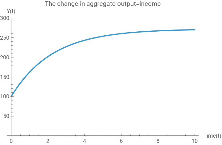
As before, equilibrium aggregate output-income grows exponentially toward its upper limit that is determined by the aggregate demand in this model economy.
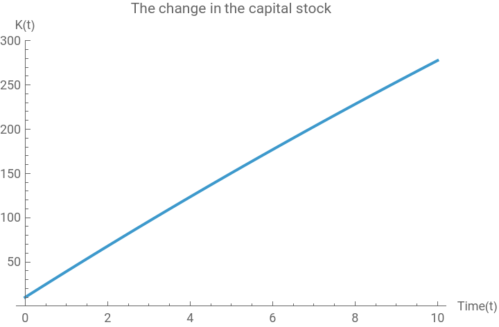
Compared to the previous session, however, we can also find the trajectory of both the productive capital stock and the government’s debt accumulation as follow:
In[]:=
sol2=RSolve[{K[t]K[t-1]+PBI-δK[t],K[0]==K0},K[t],t]
Out[]=
{{K[t]-500.(3.-3.-0.02)}}
-1.t
52.02
1.t
1.02
t
2.
2.t
5.
1.t
1.02
t
51.
1.t
51.
In[]:=
Plot[K[t]/.sol2,{t,0,10},PlotRange->{0,300},PlotLabel->"The change in the capital stock",AxesLabel->{"Time(t)","K(t)"}]
Out[]=
In[]:=
Y[t_]:=-10.88888888888889`(25.`-25.`-9.183673469387754`);sol3=RSolve[{Debt[t]Debt[t-1]+τY[t-1]-(G+TR),Debt[0]==Debt0},Debt[t],t]
-1.`t
39.0625`
1.`t
1.5625`
4.`t
2.`
1.`t
1.5625`
t
25.`
1.`t
25.`
Out[]=
{{Debt[t]-0.153086(559.677-625.+36.2903t)}}
-2.t
5.
2.t
5.
t
16.
2.t
5.
In[]:=
Plot[Debt[t]/.sol3,{t,0,10},PlotLabel->"The change in the government's debt",AxesLabel->{"Time(t)","Debt(t)"}]
Out[]=
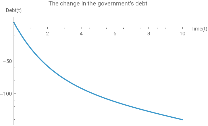
Notice that the government’s debt is falling into the negative territory. In this model setting, this means that the government sector is continuously accumulating its public debt as it engages in fiscal deficit spending over time. For common sense understanding of the increasing debt stock, however, we may need to slightly modify the previous equation for the debt accumulation as follows:
Debt[t]Debt[t-1]+(G+TR)-τY[t-1]
(
4
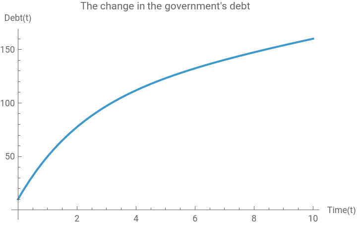
)This modified equation is conceptually the same as before (3): The government debt at time t is an increasing function of its spending flow and a negative function of its tax revenue given its debt measured a period earlier. We are using the same debt accumulation equation, but with a slightly different arrangement of two flows. Once we do this, we get the following behavior of the government debt accumulation:
In[]:=
sol4=RSolve[{Debt[t]Debt[t-1]+(G+TR)-τY[t-1],Debt[0]==Debt0},Debt[t],t]
Out[]=
{{Debt[t]0.153086(690.323-625.+36.2903t)}}
-2.t
5.
2.t
5.
t
16.
2.t
5.
In[]:=
Plot[Debt[t]/.sol4,{t,0,10},PlotLabel->"The change in the government's debt",AxesLabel->{"Time(t)","Debt(t)"}]
Out[]=
A differential equation model
A differential equation model
The model and analytical solution for equilibrium aggregate output-income
The model and analytical solution for equilibrium aggregate output-income
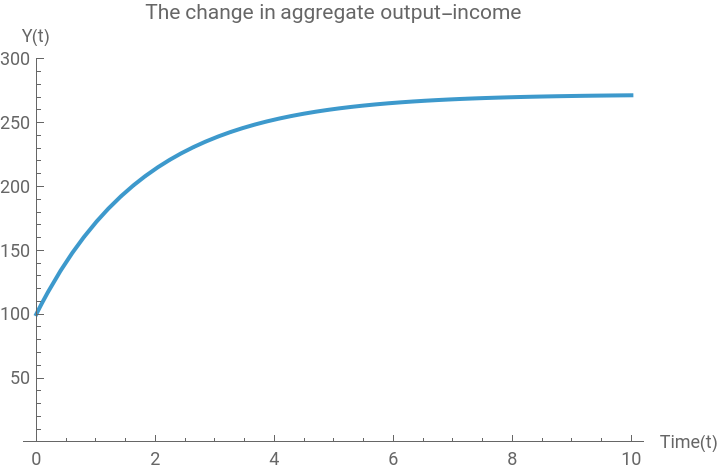
We can replicate the same behavior of both AD and Y in a differential equation model. Suppose that the change in aggregate output-income over time is induced by the force that closes the gap between aggregate demand and aggregate output-income. We can write the following differential equation for this scenario:
Y
t
where α is an adjustment parameter.
This is a linear first-order differential equation with a constant coefficient of α, a, and b. The analytical solution to this equation is:
In[]:=
Clear[α,a,b,Y,τ,PBI,G,TR,Debt,Debt0,K,K0,Y0,t,sol1,sol2];DSolve[{Y'[t]α(a+b(Y[t]-τY[t]+TR)+PBI+G-Y[t]),Y[0]==Y0},Y[t],t]//Simplify
Out[]=
Y[t](a(-1+)+(-1+)G-PBI+PBI-bTR+bTR+Y0-bY0+bY0τ)
-tα(1+b(-1+τ))
tα(1+b(-1+τ))
tα(1+b(-1+τ))
tα(1+b(-1+τ))
tα(1+b(-1+τ))
1+b(-1+τ)
A numerical example and visualization of solution curves
A numerical example and visualization of solution curves
Now suppose we have the following set of numerical values of parameters and the initial conditions. The solution curve of equilibrium aggregate output-income will be:
In[]:=
α=1.5;a=10;b=0.8;PBI=30;δ=0.02;G=50;TR=10;τ=0.2;Y0=100;K0=10;Debt0=10;sol1=DSolve[{Y'[t]α(a+b(Y[t]-τY[t]+TR)+PBI+G-Y[t]),Y[0]==Y0},Y[t],t][[1]]
Out[]=
{Y[t]272.222(-0.632653+1.)}
-0.54t
0.54t
In[]:=
Plot[Y[t]/.sol1,{t,0,10},PlotRange->{0,300},PlotLabel->"The change in aggregate output-income",AxesLabel->{"Time(t)","Y(t)"}]
Out[]=
The productive capital stock will accumulate as follows:
The government’s debt stock will accumulate as follows:
Notice that the solution curve of both Y[t] and K[t] remain the same as in the difference equation model. But the accumulation of the government’s debt stock exhibits a qualitatively different pattern from the difference equation model; it looks exponentially growing but with highly sensitive and instantaneous adjustments to the change in Y[t].
Conclusion
Conclusion
In this note, we have tried to account for the accumulation of the productive capital stock and the government’s debt by successively deriving the relevant difference/differential equation for these two stocks. The capital stock is a function of a fixed private business investment spending (inflow) and the constant depreciation (outflow), whereas the government’s debt is affected by the marginal tax revenue (outflow) and its constant fiscal spending (inflow). If the private business investment spending is greater than the depreciation, and if the government’s fixed spending is greater than its revenue, both the capital stock and the government’s debt stock increase continuously.
One can easily introduce various labor market variables such as the desired workforce, actual workforce, net hiring rate with time delay, etc., by assuming a fixed average capital-labor ratio. As the capital stock accumulates, given this average capital-labor ratio, we can expect that there will be a greater demand for labor. Depending on how fast the model economy hires new workers, given the total available labor supply, the discrepancy between the desired and actual workforce may generate a certain negative feedback on the further accumulation of the capital stock.
We can also think of additional effects of the government’s deficit spending and the resultant accumulation of its debt. For example, we can easily introduce the average rate of interest tied to the government’s deficit spending and its debt in order to account for the effect of this interest payment obligation tied to the government’s bond issuance on equilibrium aggregate output-income.
Reference
Reference
John M. Keynes, The General Theory of Employment, Money and Interest. New York: Prometheus Books, 1997 [1936].
Neva Goodwin et. al., Macroeconomics in Context, New York and London: Routledge, 2023 (The 4th edition)
Ronald Shone, An Introduction to Economic Dynamics, Cambridge University Press: 2001, pp.48-60.
Srinivas Raghavendra and Petri T. Piiroinen, An Introduction to Economic Dynamics - Modelling, Analysis and Simulation, Routledge: 2023, pp.47-60.
CITE THIS NOTEBOOK
CITE THIS NOTEBOOK
Introduction to dynamic economic models: Keynes's AD model with the capital stock and the debt
by Hee-Young Shin
Wolfram Community, STAFF PICKS, December 10, 2025
https://community.wolfram.com/groups/-/m/t/3588051
by Hee-Young Shin
Wolfram Community, STAFF PICKS, December 10, 2025
https://community.wolfram.com/groups/-/m/t/3588051