We use molecular dynamics simulation data of the CXCR7 protein. This protein is a G protein-coupled receptor (GPCRs), it scavenges chemokines and opioids, and recruit β-arrestins, so it is an atypical GPCR.
For the protein helices, we extract the spatial coordinates of atoms of alpha carbon (“CA”) and monitor how their positions evolve over time using static and dynamic graphical analysis. In parallel, we compute pairwise contact distances between protein residues and analyze how these distances fluctuate throughout the simulation trajectory.
CXCR7 Protein
CXCR7 Protein
First we import the reference structure of the CXCR7 protein, the format that contains the information of said protein is a PDB format, so we have access to the types of atoms that form the protein, as well as their positions in Cartesian coordinates. When viewing the protein, it was observed that there are different types of secondary structure in the protein, so, for the interest of this work, we only focused on studying the seven transmembrane helices.
In[]:=
cxcr0=BioMolecule;


We used the functions of the "ProteinVisualization" paclet to begin studying the structure of the protein .
In[]:=
BioMoleculePlot3D[cxcr0]
Out[]=
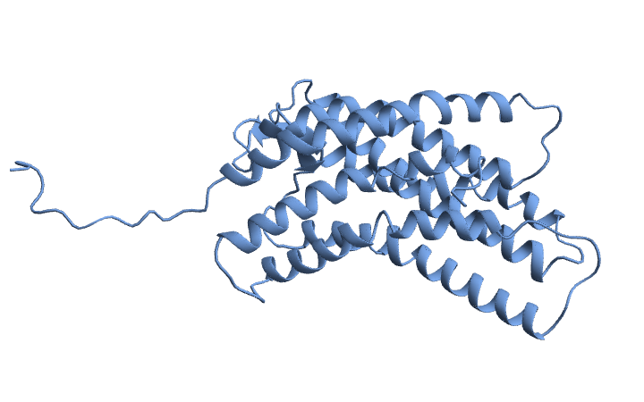
A object has many properties:
BioMolecule
cxcr0["Properties"]
Out[]=
{Assemblies,AssemblyCount,AssemblyData,AtomCoordinates,AtomCoordinateValues,AtomCount,AtomCounts,AtomicSymbols,AtomLabels,AuthorChainIDs,AuthorResidueIDs,BFactors,BioSequence,BioSequences,ChainCount,ChainIDs,Chains,ChainTypes,Citations,ComputedStructureQ,CrystallographicSpaceGroup,Helices,ModelCount,Models,Name,PDBStructureID,PeptideTorsionAngles,PolymerChainCount,PolymerChainIDs,PolymerChains,RamachandranAngles,ResidueAbbreviations,ResidueCount,ResidueCounts,ResidueIDs,Sheets,UnitCellAngles,UnitCellLengths}
The property gives a list of residue ranges in each chain that are α-helical.
"Helices"
cxcr0["Helices"]
Out[]=
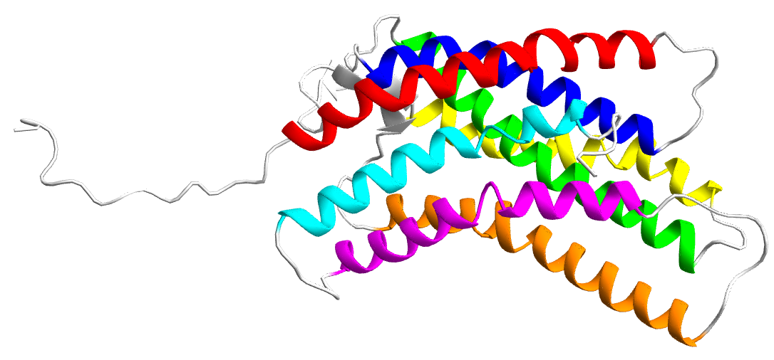
A{{19,39},{40,44},{45,52},{61,87},{96,129},{135,140},{141,145},{147,151},{152,164},{189,199},{200,204},{205,223},{234,245},{248,262},{269,286},{289,295}}
This information allowed us to visualize the alpha helices of the protein and define the contiguous range of amino acid residues for each helix.
In[]:=
BioMoleculePlot3D[cxcr0,ColorRules->{{"A",Alternatives@@Range[19,52]}->Red,{"A",Alternatives@@Range[61,87]}->Blue,{"A",Alternatives@@Range[96,129]}->Green,{"A",Alternatives@@Range[135,164]}->Yellow,{"A",Alternatives@@Range[189,223]}->Orange,{"A",Alternatives@@Range[234,262]}->Magenta,{"A",Alternatives@@Range[269,295]}->Cyan,{"A",_}->LightGray},ImageSize->Large(*,SphericalRegion->True*)]
Molecular Dynamics
Molecular Dynamics
To investigate the conformational behavior of the protein within a cell membrane environment, molecular dynamics (MD) simulations were performed using the CHARMM force field, a well established parameter set for modeling biomolecular systems with atomic level accuracy. CHARMM (Chemistry at HARvard Macromolecular Mechanics) provides detailed representations of bonded and non-bonded interactions including bond stretching, angle bending, torsions, van der Waals forces, and electrostatics making it particularly suitable for simulating the flexibility and stability of proteins in explicit solvent and lipid environments. The system was prepared for simulation by embedding the protein model in a fully hydrated lipid bilayer model, followed by the addition of ions to achieve electrostatic neutrality and physiological ionic strength. After energy minimization and equilibration steps to relax the system and remove steric clashes, a production MD simulation was carried out for a total of 1 microsecond. This timescale is long enough to capture a variety of biologically relevant motions, including local side chain rearrangements, helix bending or tilting, and coordinated domain shifts that occur on the nanosecond to microsecond range. The simulation was conducted under constant temperature and pressure (NPT ensemble), using a time step of 2 femtoseconds and periodic boundary conditions to mimic the infinite membrane environment. The resulting trajectory provides detailed atomic positions at regular intervals over the entire microsecond, allowing for in depth post simulation analysis of the structural dynamics and inter-helical interactions within the protein . All this was done before arriving at the Summer School.
Whole Protein Motion
Whole Protein Motion
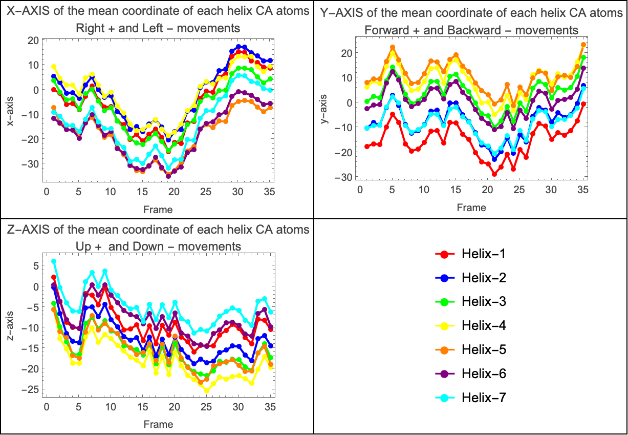
Using the filtered positional data of the Cα atoms for each helix, we computed the average coordinates along each Cartesian axis. This resulted in three separate plots—one for each axis—illustrating how the protein shifted right or left (x-axis), forward or backward (y-axis), and up or down (z-axis) throughout the simulation. Since the protein is embedded within a lipid bilayer, its movements are constrained by the surrounding membrane molecules. To further explore the dynamics, we analyzed whether the average coordinates of the helices were coupled across the axes. This led to the generation of three additional plots, each capturing the collective motion of the helices along a specific axis.
The graphs reveal that the alpha helices exhibit coordinated, or coupled, movement throughout the simulation. In each of the three plots—corresponding to the X, Y, and Z Cartesian axes—we observe that the average positional trajectories of the helices follow similar trends over time. This indicates that the helices are not moving independently; instead, they tend to shift together in the same direction along each axis. Such coupling suggests a level of structural coherence within the transmembrane domain, likely influenced by both the intrinsic stability of the protein and the constraining effect of the surrounding lipid bilayer. In other words, rather than fluctuating randomly, the helices maintain a degree of synchronized motion, pointing to potential functional or mechanical relationships between them.
In[]:=
Grid[{{plotxaxis,plotyaxis},{plotzaxis,legend}},Frame->All]
Out[]=
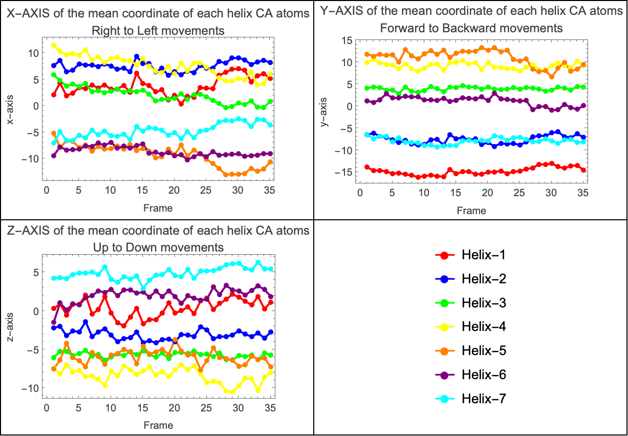
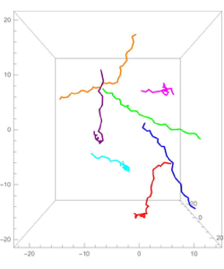
The coordinates of the alpha carbon atoms (Cα) effectively capture the backbone path of each helix, providing a simplified yet informative representation of its shape. Based on this, we approximated a line passing through the centroid of each transmembrane alpha helix to better understand their orientation and relative displacement over time. By plotting these centroid based lines in a 3D graph, we were able to visualize the spatial arrangement of the helices and how they evolve during the simulation. This approach offers a clearer view of the protein’s overall structural dynamics, highlighting shifts in orientation and potential coordinated rearrangements among helices within the membrane environment. The following graphs show how the propellers move relative to the center of mass of the system.
In[]:=
ListLinePlot[differenceBetweenCenters[[All,All,#[[1]]]],Mesh->All,PlotStyle->Thread[Directive[PointSize[0.02],helixColors]],Frame->True,FrameLabel->{"Frame",#[[2]]},PlotLabel->#[[3]],ImageSize->300]&/@{{1,"x-axis","X-AXIS of the mean coordinate of each helix CA atoms\nRight to Left movements"},{2,"y-axis","Y-AXIS of the mean coordinate of each helix CA atoms\nForward to Backward movements"},{3,"z-axis","Z-AXIS of the mean coordinate of each helix CA atoms\nUp to Down movements"}}//Append[legend]//Partition[#,2]&//Grid[#,Frame->All]&
Out[]=
Transmembrane Helices
Transmembrane Helices
Two approximations were used for the next part of the analysis. The first used the moving average of the alpha carbon coordinates, however, it was unsatisfactory because the line became increasingly shorter as the size of the moving average window was increased, and would not represent the full length of the helix.
This second approximation is used to show the shape of each alpha helix in the protein using only the alpha carbon (Cα) atoms. First, it calculates points between groups of three Cα atoms by taking the average position of the first and last atoms in each group. These average points create a smooth curve that goes through the center of each helix. Then, it draws 3D plots for each helix . In each plot, we see two lines: one showing the real positions of the Cα atoms, and another showing the smooth line that represents the central curve of the helix. This helps us better understand the position and shape of each helix during the simulation.
Out[]=
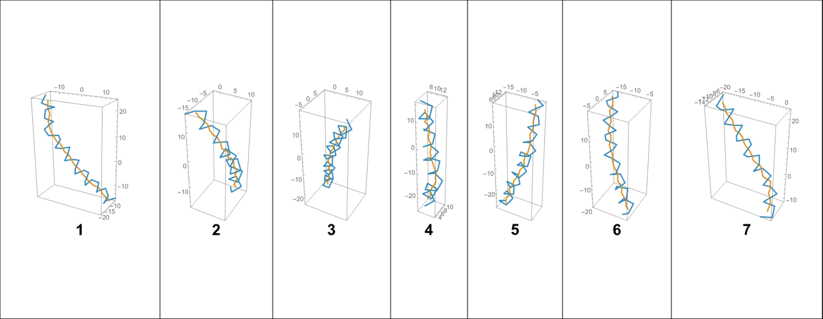
By approximating a line that passes through the centroid of each alpha helix, a 3D plot was generated to visualize their spatial arrangement relative to the system’s center of mass. This representation provides insight into how each helix is positioned and oriented within the protein structure, and how these orientations evolve throughout the simulation. Referencing the center of mass allows for a more accurate interpretation of global versus local motions within the membrane-embedded protein.
Out[]=
Using the contact matrix, we constructed a dynamic visualization that captures how the interactions between alpha helices evolve over the course of the simulation. This representation makes it possible to visualize not just static contacts, but also how these interactions fluctuate and reorganize over time. It is particularly interesting to observe the dynamic nature of these contacts, as they reveal transient associations, stable interfaces, and possible shifts in helix-helix connectivity that may be functionally relevant to the behavior of the protein within the membrane.
Atom-level Motion
Atom-level Motion
For the last part of the analysis we consider the Euclidean distance for each CA atom represented by a sphere, and on a color scale, where green means a minimal change in the atom' s position and red a large change in position .
Initialization
Initialization
Acknowledgment
Acknowledgment
I am grateful to WSS, Bob Nachbar, Paul Abbott, Lina Ruiz and Stephen Wolfram, and all the other people who made this possible .
Cite this Notebook
Cite this Notebook