PI Controller Tuning : Mathematica vs. Simulink
Authors: Housam Binous and Ahmed Bellagi
PI Controller Tuning : Mathematica vs. Simulink
Authors: Housam Binous and Ahmed Bellagi
Authors: Housam Binous and Ahmed Bellagi
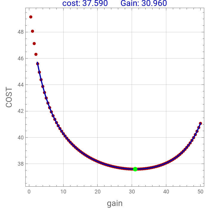
We perform PI controller tuning by adopting a Cost function given by Dr. Steve Brunton. This cost function is designed to minimize the ISE while penalizing high values of the manipulated variable or u. Excellent agreement is found between Simulink model and our Mathematica coding.
Reference:
https://www.youtube.com/watch?v=S5C_z1nVaSg
Reference:
https://www.youtube.com/watch?v=S5C_z1nVaSg
MATHEMATICA code below uses FindMinimum to fetch best PI controller parameters based on the CRITERIA by Dr. Steve Brunton. We assume that the controller transfer function is : Gc = KP + TAUI/s with TAUI = 0.2
In[]:=
Gc[KP_?NumericQ,TAUI_?NumericQ]:=KP+TAUI/s;GT=1/(s+1)/(s+2)/(s+3)
Out[]=
1
(1+s)(2+s)(3+s)
In[]:=
G[KP_?NumericQ,TAUI_?NumericQ]:=GTGc[KP,TAUI]/(1+GTGc[KP,TAUI])
In[]:=
Gu[KP_?NumericQ,TAUI_?NumericQ]:=Gc[KP,TAUI]/(1+GTGc[KP,TAUI])
In[]:=
y[KP_?NumericQ,TAUI_?NumericQ]:=InverseLaplaceTransform[1/sG[KP,TAUI],s,t]//Chop;
In[]:=
u[KP_?NumericQ,TAUI_?NumericQ]:=InverseLaplaceTransform[1/sGu[KP,TAUI],s,t]//Chop;
In[]:=
f1[KP_?NumericQ,TAUI_?NumericQ]:=Re[Quiet@NIntegrate[(1-y[KP,TAUI])^2+0.001(u[KP,TAUI])^2,{t,0,1000}]//Chop];
In[]:=
w1=FindMinimum[f1[q,0.2],{q,1.5,1.4}]
Out[]=
{37.5935,{q30.9646}}
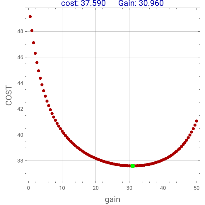
Let us plot the cost function versus KP
In[]:=
data=Table[{KP,f1[KP,0.2]},{KP,0.5,50,0.5}]
Out[]=
{{0.5,49.145},{1.,48.0608},{1.5,47.1239},{2.,46.3063},{2.5,45.5868},{3.,44.9489},{3.5,44.3796},{4.,43.8684},{4.5,43.4071},{5.,42.9888},{5.5,42.6078},{6.,42.2596},{6.5,41.9401},{7.,41.646},{7.5,41.3746},{8.,41.1234},{8.5,40.8903},{9.,40.6736},{9.5,40.4716},{10.,40.2831},{10.5,40.1068},{11.,39.9417},{11.5,39.7868},{12.,39.6413},{12.5,39.5046},{13.,39.3758},{13.5,39.2545},{14.,39.1401},{14.5,39.0322},{15.,38.9303},{15.5,38.834},{16.,38.7431},{16.5,38.6571},{17.,38.5758},{17.5,38.4989},{18.,38.4263},{18.5,38.3576},{19.,38.2927},{19.5,38.2315},{20.,38.1737},{20.5,38.1192},{21.,38.068},{21.5,38.0197},{22.,37.9745},{22.5,37.9321},{23.,37.8924},{23.5,37.8555},{24.,37.8211},{24.5,37.7893},{25.,37.7601},{25.5,37.7332},{26.,37.7088},{26.5,37.6868},{27.,37.6671},{27.5,37.6498},{28.,37.6348},{28.5,37.6221},{29.,37.6117},{29.5,37.6036},{30.,37.5979},{30.5,37.5945},{31.,37.5935},{31.5,37.5948},{32.,37.5987},{32.5,37.605},{33.,37.6138},{33.5,37.6253},{34.,37.6394},{34.5,37.6563},{35.,37.676},{35.5,37.6987},{36.,37.7244},{36.5,37.7534},{37.,37.7857},{37.5,37.8214},{38.,37.8608},{38.5,37.9041},{39.,37.9515},{39.5,38.0032},{40.,38.0594},{40.5,38.1205},{41.,38.1868},{41.5,38.2587},{42.,38.3366},{42.5,38.4209},{43.,38.5121},{43.5,38.6109},{44.,38.7179},{44.5,38.8338},{45.,38.9595},{45.5,39.096},{46.,39.2443},{46.5,39.4057},{47.,39.5818},{47.5,39.7741},{48.,39.9848},{48.5,40.2162},{49.,40.4711},{49.5,40.7528},{50.,41.0653}}
In[]:=
p=ListPlot[data,PlotRangeAll,FrameTrue,AspectRatio1,GridLinesAutomatic,PlotStyle{Thick,PointSize[0.0175],Darker@Red},Epilog{Green,PointSize[0.025],Point[{q/.w1[[2]],w1[[1]]}]},ImageSize{350,350},PlotLabelRow[{Style["cost: ",14,Darker@Blue],Style[NumberForm[w1[[1]],{4,3}],14,Darker@Blue]," ",Style["Gain: ",14,Darker@Blue],Style[NumberForm[q/.w1[[2]],{4,3}],14,Darker@Blue]}],FrameLabel{Style["gain",14],Style["COST",14]}]
Out[]=
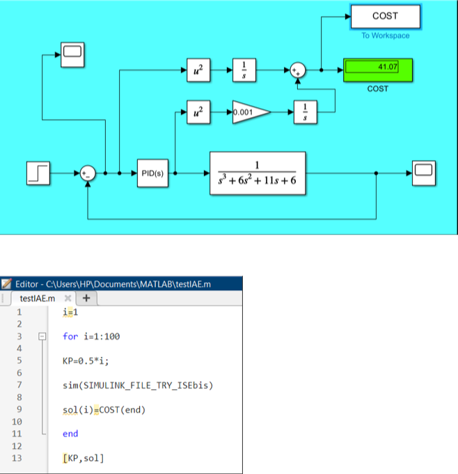
Below we provide the values of the cost function versus KP obtained using the following Simulink model and the Matlab script.
In[]:=
In[]:=
dataSIMULINK={{0.5000,49.1450},{1.0000,48.0608},{1.5000,47.1239},{2.0000,46.3063},{2.5000,45.5868},{3.0000,44.9489},{3.5000,44.3796},{4.0000,43.8684},{4.5000,43.4071},{5.0000,42.9888},{5.5000,42.6078},{6.0000,42.2596},{6.5000,41.9401},{7.0000,41.6460},{7.5000,41.3746},{8.0000,41.1234},{8.5000,40.8903},{9.0000,40.6736},{9.5000,40.4716},{10.0000,40.2831},{10.5000,40.1068},{11.0000,39.9417},{11.5000,39.7868},{12.0000,39.6413},{12.5000,39.5046},{13.0000,39.3758},{13.5000,39.2545},{14.0000,39.1401},{14.5000,39.0322},{15.0000,38.9303},{15.5000,38.8340},{16.0000,38.7431},{16.5000,38.6571},{17.0000,38.5758},{17.5000,38.4989},{18.0000,38.4263},{18.5000,38.3576},{19.0000,38.2927},{19.5000,38.2315},{20.0000,38.1737},{20.5000,38.1192},{21.0000,38.0680},{21.5000,38.0197},{22.0000,37.9745},{22.5000,37.9321},{23.0000,37.8924},{23.5000,37.8555},{24.0000,37.8211},{24.5000,37.7893},{25.0000,37.7601},{25.5000,37.7332},{26.0000,37.7088},{26.5000,37.6868},{27.0000,37.6671},{27.5000,37.6498},{28.0000,37.6348},{28.5000,37.6221},{29.0000,37.6117},{29.5000,37.6036},{30.0000,37.5979},{30.5000,37.5945},{31.0000,37.5935},{31.5000,37.5948},{32.0000,37.5987},{32.5000,37.6050},{33.0000,37.6138},{33.5000,37.6253},{34.0000,37.6394},{34.5000,37.6563},{35.0000,37.6760},{35.5000,37.6987},{36.0000,37.7244},{36.5000,37.7534},{37.0000,37.7857},{37.5000,37.8214},{38.0000,37.8608},{38.5000,37.9041},{39.0000,37.9514},{39.5000,38.0032},{40.0000,38.0594},{40.5000,38.1205},{41.0000,38.1868},{41.5000,38.2587},{42.0000,38.3366},{42.5000,38.4209},{43.0000,38.5121},{43.5000,38.6109},{44.0000,38.7178},{44.5000,38.8338},{45.0000,38.9595},{45.5000,39.0959},{46.0000,39.2443},{46.5000,39.4057},{47.0000,39.5818},{47.5000,39.7741},{48.0000,39.9848},{48.5000,40.2162},{49.0000,40.4710},{49.5000,40.7528},{50.0000,41.0653}};
In[]:=
Show[p,ListPlot[dataSIMULINK,Joined->True,PlotStyle->Darker@Blue]]
Out[]=