Introduction
Introduction
In the era of COVID-19, where the world has been turned upside down by a pandemic, many countries are utilizing contact tracing to reduce the spread of the virus and “flatten the curve” allowing hospitals to keep up with the number of infected people. For my simulation I implemented my contact tracing such that when a person is infected, a list of people that they have been in contact with is put together, and each of those people isolate themselves from the rest of the network for a certain period of time in order to inhibit the spread of the infection. In my project, I utilized undirected graphs in the Wolfram Language to create a simulation of the spread of a virus, and used this to explore how different levels of contact tracing can slow the spread of infections through a social network over time. Working with mentors, I created this project as a part of the 2020 Wolfram High School Summer Camp.
Initializing the elements
Initializing the elements
In order to model the spread of a virus, the first challenge is to try to model a social network, where each node represents a person and the edges represent interactions between them. We can model a social network with a random graph to run our simulation on. For my social network, I used a Watts-Strogatz graph with a rewiring probability of 0.2. Watts-Strogatz graphs have higher levels of clustering than a regular random graph and therefore represent a social network reasonably well. Of course, we will never be able to graph every instance of human contact, so this approximation is not perfect, but it does allow us to analyze contact tracing and its effectiveness.
Generates the graph for arbitrary social network:
In[]:=
nodes=250;g=RandomGraph@WattsStrogatzGraphDistribution[nodes,0.2]
Out[]=
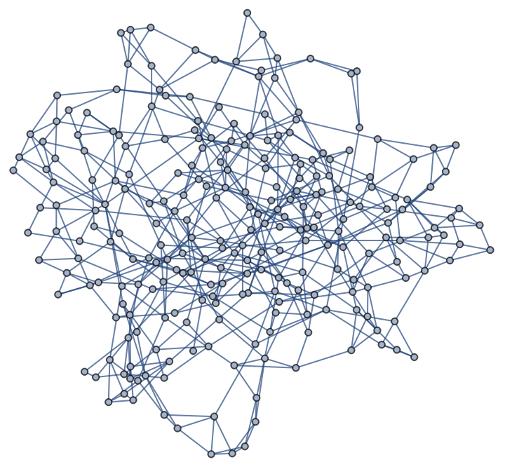
We also assign weight for each edge in the graph. These weights represent how “close” the two nodes were in their contact and it’s used to manipulate the probability of how likely a node is to get infected from another node. For example, a person that you shake hands with would have a much lower weighting than someone that you live with. For my simulation, I set these values between 0.7 and 1.3 because I found that larger ranges gave me data that wasn’t consistent, and the infection could sometimes “fizzle out” in the first few steps.
Assigns random edge weights:
In[]:=
g=SetProperty[g,EdgeWeightNormal@AssociationThread[EdgeList[g],Table[RandomReal[{0.7,1.3}],EdgeCount[g]]]];
Defines some variables we will need: mortalityProb, which allows us to change the probability that any infected node will die from the virus, recoveryTime, which is the number of cycles after which a node will recover, and quarantineTime, which is the number of cycles a node stays quarantined:
In[]:=
mortalityProb=0.3;recoveryTime=10;quarantineTime=5;
As the last step to initialization, we can infect two nodes and initialize the counter association for quarantined nodes. We infect two nodes for the same reason we have a limited range in our edge weighting - because these factors and the relatively small number of connections each node means that the infection can sometimes die out in the first few steps and we can get outliers in our data.
Infect two nodes and create an association for the quarantined nodes:
iCounter=Association[#recoveryTime&/@RandomSample[VertexList[g],2]];qCounter=<||>;
Simulating the spread
Simulating the spread
In order to simulate the spread of the virus, we can create a function that simulates one exposure cycle, called step[] in this project. Due to the varying nature of an exposure cycle in different social networks, and how new COVID is, in this project, we'll be leaving a "step" as an arbitrary length of time. The length of an exposure cycle also defines the "recovery time" and time spent in quarantine for every node that gets traced, which, here, are arbitrarily defined as 10 and 5 cycles respectively. Each of the following snippets of code are parts of the bigger step[] function, but won’t run on their own.
iCounter and qCounter are Associations for which the keys are the indexes of the infected and quarantined nodes, and the values are the number of iterations they have left as either infected or quarantined. They are originally set to the recoveryTime and quarantineTime. Each step, the “counter” values are reduced by one, until they reach 0, when they are removed from the association and returned to the rest of the population. As each of the nodes recover and exit iCounter, they’re also added to iList which simulates gaining immunity, which reduces their chance of getting the virus again.
Decrements the counters, "recovers" and "de-quarantines" nodes at the end of their counters, and updates the immunity list:
In[]:=
If[qCounter[#]0,qCounter=KeyDrop[qCounter,#],qCounter[#]-=1]&/@Keys[qCounter];If[iCounter[#]0,iCounter=KeyDrop[iCounter,#];iList=Append[iList,#],iCounter[#]-=1]&/@Keys[iCounter];
There is also a “mList” containing all dead nodes, representing all the nodes that die from the virus.
Each step, some small subset of the infected nodes get dropped from the association and added to this list of "dead" nodes:
In[]:=
If[RandomReal[{0,recoveryTime}]<mProb,iCounter=KeyDrop[iCounter,#];mList=Append[mList,#],Nothing]&/@Keys[iCounter];mList=Flatten[mList];
From the association of infected nodes, a list of all the nodes they are connected to, called "contacts" is created. Nodes that are already infected, quarantined, or dead are not included in this list:
In[]:=
contacts=Complement[VertexOutComponent[g,Flatten[Complement[Keys[iCounter],Keys[qCounter]]],1],Union[Keys[iCounter],Keys[qCounter],mList]];
Some subset of the contacts get traced and quarantined based off of the tracing probability (traProb):
traced=RandomSample[contacts,Round[traProb*Length[contacts]]];(qCounter[#1]=#2)&@@@(#5&/@traced);
For each infected node, each of the nodes it is connected to is added to the list of "infected" nodes with a probability based on the transmission probability (transProb) and the edge weight of the edge between the two endpoints:
infected={};Map[Function[node,If[RandomReal[{0,1}]<transProb*PropertyValue[{g,node#},EdgeWeight],infected=AppendTo[infected,node],Nothing]],VertexOutComponent[g,#,1]]&/@Complement[Keys[iCounter],Keys[qCounter]];
Then, all of the nodes that are already infected, quarantined, or dead are removed from the list. Of the infected, those that are immune also get removed with an 80% probability before each element of that list gets added to the association. totalInfect keeps track of the total number of infections so far:
infected=Complement[infected,Union[Keys[iCounter],Keys[qCounter],mList]];infected=Complement[infected,RandomSample[iList,Round[0.8*Length[iList]]]];totalInfect+=Length[infected];
As the last step to our function, we can return the current number of infections, total infections, and number of deaths, and recursively call our function again for the next simulation step:
l={Length[Keys[iCounter]],totalInfect,Length[mList]};Join[{l},step[transProb,traProb,mProb,g,qCounter,iCounter,mList,iList,totalInfect,n-1]];
Full definition of step[]
Full definition of step[]
Visualizing the data
Visualizing the data
We can now use the data from our function step[] to create some very interesting plots and visuals to explore how the degree of contact tracing and how infectious the virus is affects its spread.
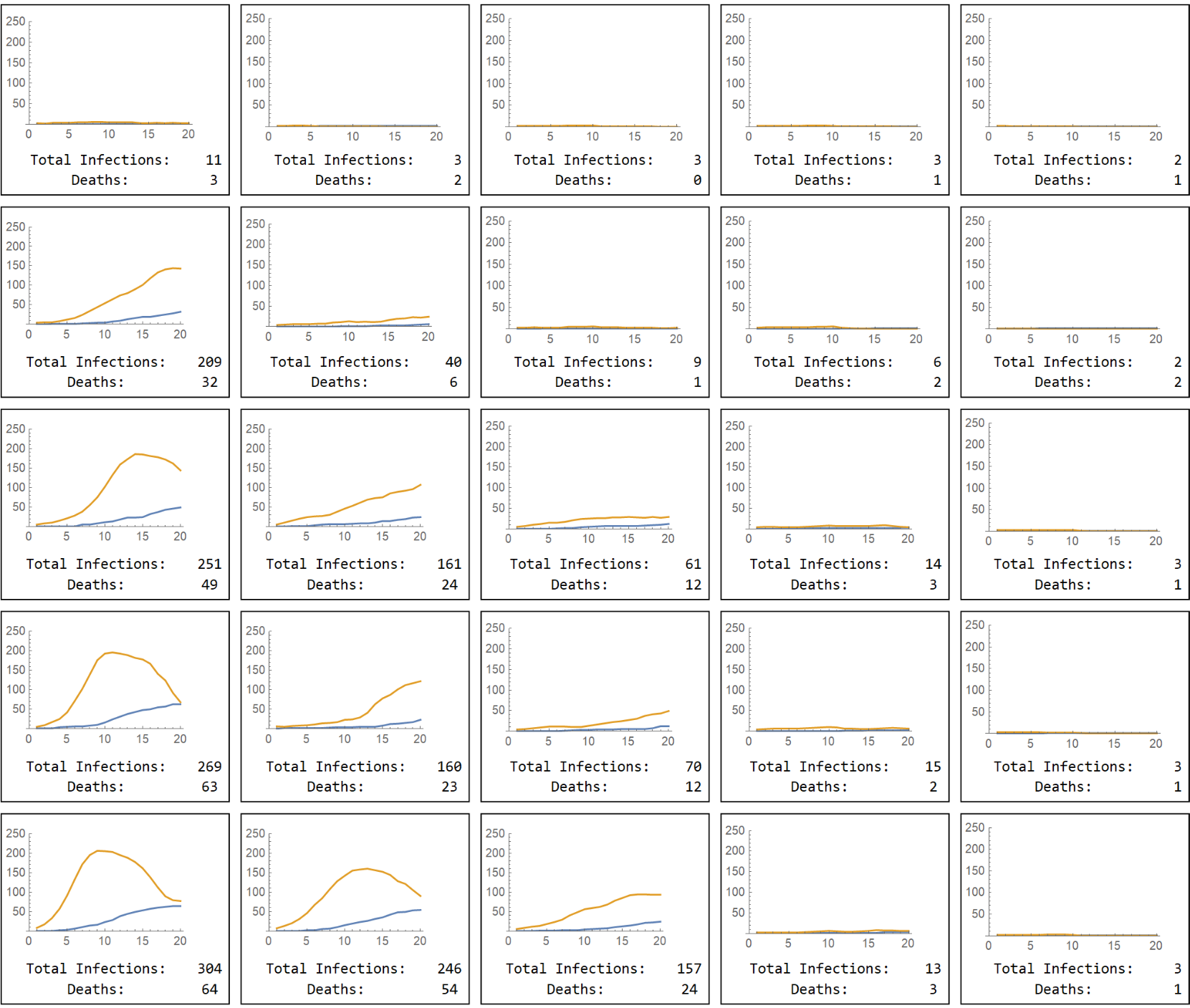
As the "infectiousness" or transmission probability (rows) and the probability of being able to trace the contacts of cases (columns) vary, the number of infections and deaths change:
iCounter=Association[#recoveryTime&/@RandomSample[VertexList[g],2]];qCounter=<||>;mortalityList={};immunityList={};Grid[Table[data=step[transmit,trace,mortalityProb,g,qCounter,iCounter,mortalityList,immunityList,Length[Keys[iCounter]],20];Framed@Grid[{{ListLinePlot[{Flatten[Last/@data],Flatten[First/@data]},PlotRange{{0,nodes}}]},{"Total Infections:",(Last[data])[[2]]},{"Deaths:",Last@Last[data]}}],{transmit,0.1,0.9,0.2},{trace,0.1,0.9,0.2}]]
Out[]=
We can change the return of step[] slightly to see how the infection spreads on a graph. For the example below, I chose a graph with fewer nodes, to make it easier to see. Here, red nodes are infected, and orange nodes are infected but quarantined, so the infection can't spread from them:
g=RandomGraph@WattsStrogatzGraphDistribution[20,0.2];g=SetProperty[g,EdgeWeightNormal@AssociationThread[EdgeList[g],Table[RandomReal[{0.7,1.3}],EdgeCount[g]]]];iCounter=Association[#recoveryTime&/@RandomSample[VertexList[g],1]];qCounter=<||>;ListAnimate[stepGraph[0.6,0.5,mortalityProb,g,qCounter,iCounter,mortalityList,immunityList,Length[Keys[iCounter]],10],AnimationRunningFalse,SaveDefinitionsTrue]
Comparing this to the spread on the same graph with the same transmission probability, but a slightly lower tracing results in a much higher rate of spread through the network:
Conclusion
Conclusion
Ideally, of course, 100% contact tracing is extremely effective and a very valuable tool in reducing the fatality of a virus after it enters a social network. However, this is often not feasible given all of the small interactions between people in a day, and the resources needed to do this contact tracing. Based off the graphs, we can see that even 50% effective contact tracing reduces the deaths by 50-70%. It also significantly "flattens the curve" by reducing new cases per day, which should allow medical staff to continue caring for each patient with the resources they need. At 70% contact tracing, the curve flattens even further and gets close to the results of 100% contact tracing. Based off of this simulation, 50-70% effective contact tracing seems to be the "sweet spot" of having huge positive effects on the spread of the virus, but also being easy to implement.
Next Steps
Next Steps
There are definitely more steps to making this simulation more accurate. While I didn’t explore this variable in my simulation, the range of these edge weights could also be used to explore the effects of social distancing on an infection. If each node is an endpoint to only one or two high-weighted edges and all the rest are low because of precautions like wearing masks and maintaining distance, it would be very interesting to see how the infection curves change. This simulation also assumes that nobody starts with any level of immunity, and everyone maintains perfect quarantines. In a real pandemic, access to beds in hospitals and medical equipment is also a key factor in its mortality rate, which this simulation doesn't account for. The total number of deaths is dependant on the slope of the infections curve and how it relates to how fast medical equipment can be produced and freed up for incoming patients. Beyond a certain number of cases per day, the mortality rate would go up dramatically because each of the patients wouldn't have access to the doctors and medical care they needed. There is much to be done with this project, but we can still use it to clearly see what an important effect contact tracing and quarantining has on inhibiting the spread of a virus through a social network.