Vertical Laminar Flow of Bingham Liquid Film
Authors: Housam Binous and Ahmed Bellagi
Vertical Laminar Flow of Bingham Liquid Film
Authors: Housam Binous and Ahmed Bellagi
Authors: Housam Binous and Ahmed Bellagi
Reference:
H . Binous, Introducing non - Newtonian fluid mechanics computations with Mathematica® in the undergraduate curriculum, Chemical Engineering Education, 41 (1), pp . 59 - 64, 2007.
H . Binous, Introducing non - Newtonian fluid mechanics computations with Mathematica® in the undergraduate curriculum, Chemical Engineering Education, 41 (1), pp . 59 - 64, 2007.
Acknowledgement :
Since in this laminar flow problem we have split boundary conditions. Problem’s resolution is based on the Shooting Method developed in Mathematica by Professor Brian Higgins (University of California, Davis).
Since in this laminar flow problem we have split boundary conditions. Problem’s resolution is based on the Shooting Method developed in Mathematica by Professor Brian Higgins (University of California, Davis).
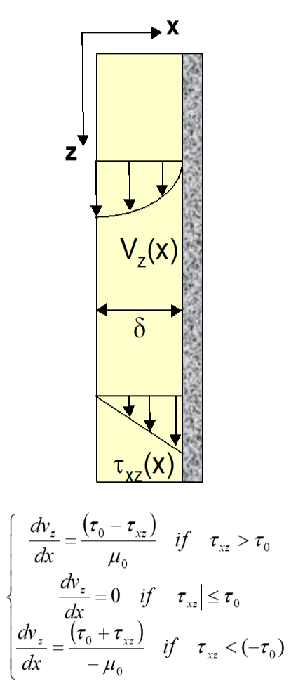
Vertical Flow of Bingham liquid film
Vertical Flow of Bingham liquid film
In[]:=
g=9.81;ρ=950;=5;=0.15;δ=0.005;
τ
0
μ
0
In[]:=
system[Ω_]={D[[x],{x,1}]ρg,D[[x],{x,1}]If[Abs[[x]]≤,0,If[[x]>,(-[x])/,-(+[x])/]],[0]0,[0]Ω};myODEsoln[Ω_]:=NDSolve[system[Ω],{,},{x,0,δ}]yend[Ω_?NumericQ]:=Flatten[([r]/.myODEsoln[Ω])/.rδ]bc=FindRoot[yend[Ω]0,{Ω,0,0.5}][[1,2]];
τ
xz
v
z
τ
xz
τ
0
τ
xz
τ
0
τ
0
τ
xz
μ
0
τ
0
τ
xz
μ
0
τ
xz
v
z
v
z
τ
xz
v
z
In[]:=
sol1=myODEsoln[bc]
Out[]=
InterpolatingFunction,InterpolatingFunction
v
z


τ
xz

In[]:=
pos=x/.FindRoot[Abs[[x]/.sol1]==,{x,0.0005}]
τ
xz
τ
0
Out[]=
0.000536512
In[]:=
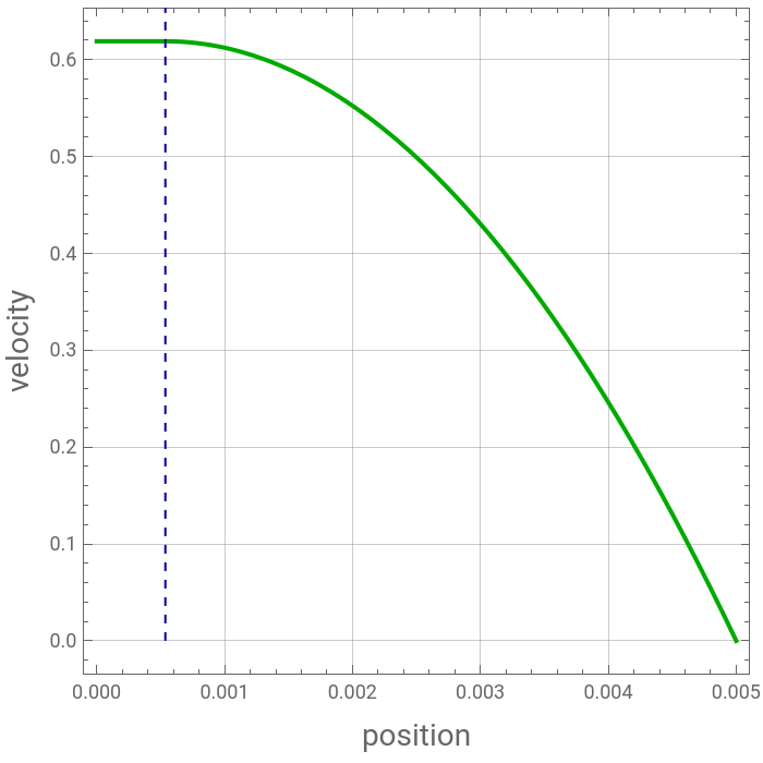
plt1=Plot[[x]/.sol1,{x,0,δ},PlotStyle{Thick,Darker@Green},Frame->True,AspectRatio->1,FrameLabel->{Style["position",14],Style["velocity",14]},GridLines->Automatic,ImageSize->350{1,1},Epilog->{Darker@Blue,Dashed,Line[{{pos,0},{pos,0.72}}]}]
v
z
Out[]=
In[]:=
plt2=Plot[[x]/.sol1,{x,0,δ},PlotStyle{Thick,Darker@Blue},Frame->True,AspectRatio->1,FrameLabel->{Style["position",14],Style["shear stress",14]},GridLines->Automatic,ImageSize->350{1,1}]
τ
xz
Out[]=
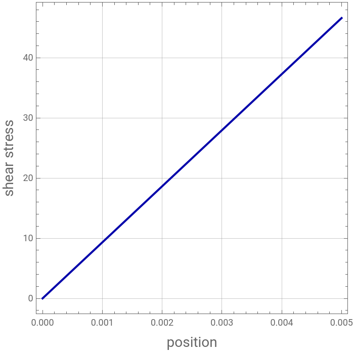
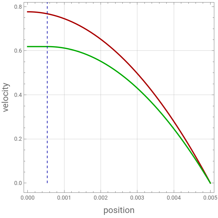
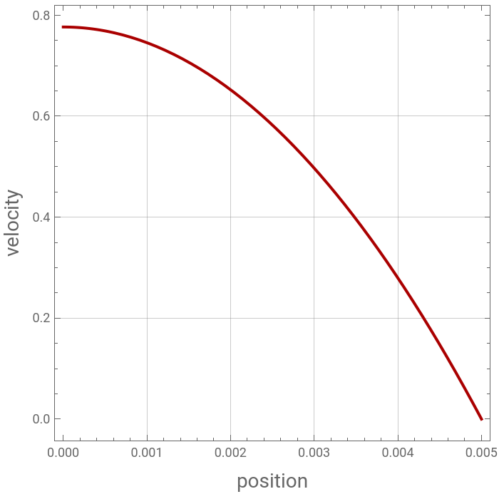
Comparison with Newtonian fluid velocity profile obtained using the analytical solution:Velocity profile for the Bingham fluid is flat near the surface of the liquid film. In fact, only when [x]>, we have a non zero velocity gradient as indicated by the blue dashed line. This behavior is typical of Bingham fluids.
v=1-
ρg
2
δ
2
μ
0
2
x
δ
τ
xz
τ
0
In[]:=
v
analytical
μ
0
In[]:=
plt3=Plot[[x],{x,0,δ},PlotStyle{Thick,Darker@Red},Frame->True,AspectRatio->1,FrameLabel->{Style["position",14],Style["velocity",14]},GridLines->Automatic,ImageSize->350{1,1}]
v
analytical
Out[]=
In[]:=
Plot[[x],[x]/.sol1,{x,0,δ},PlotStyle{{Thick,Darker@Red},{Thick,Darker@Green}},Frame->True,AspectRatio->1,FrameLabel->{Style["position",14],Style["velocity",14]},GridLines->Automatic,ImageSize->350{1,1},PlotLegends->{Style["Newtonian",14,Darker@Red],Style["Bingham",14,Darker@Green]},Epilog->{Darker@Blue,Dashed,Line[{{pos,0},{pos,0.82}}]}]
v
analytical
v
z
Out[]=