ABSTRACT (original article): The envelope theory is a reliable and easy to implement method to solve time independent Schrödinger-like equations (eigenvalues and eigenvectors). It is particularly useful to solve many-body systems since the computational cost is independent from the number of particles. The purpose of this paper is twofold. First, we want to make known a method that is probably too little used. Second, we also want to show that this method can be used as a pedagogical tool, thanks to its simplicity and the reliable results that can be obtained. To reach these goals, the envelope theory is applied to a simple problem in one dimension, the soft-Coulomb potential , characterised by a bias distance $d$. Such interaction is used for the study of excitons, electron-hole bound pairs where the two charges are kept separated in two different one-dimensional regions (quantum wires). In addition to its physical interest, this system has never been treated with the envelope theory. CITATION (original article): Claude Semay and Maud Balcaen, The envelope theory as a pedagogical tool, Eur. J. Phys. 44 (2023) 035401. https://doi.org/10.1088/1361-6404/acbe7d
-k+
2
x
2
d
Figure 1
Figure 1
The soft-Coulomb potential for D = 2 (solid black) with the Coulomb potential (dashed gray) and the quadratic potential with D = 2 (dot-dashed gray). All quantities are dimensionless.
In[]:=
d=2;(*dimensionlessparameterD*)plt=Plot-+,-,-+,{x,-6,6},PlotRange->{Automatic,{-1,0.5}},PlotStyle->{{Black},{Gray,Dashed},{Gray,DotDashed}},AxesLabel->{x,V[x]},LabelStyle->Medium,PlotLegends->Placed[{"soft-Coulomb","Coulomb","quadratic"},After]
1
2
x
2
d
1
Abs[x]
1
d
2
x
2
3
d
Out[]=
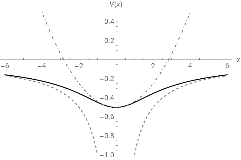


Figure 2
Figure 2
Lowest dimensionless energies for H with D = 2: accurate values obtained with the FGH method (black triangle) and upper bounds from the ET (gray diamond). The exact energies for (gray circle) and with D = 2 (gray square) are also indicated.
H
C
H
HO
Computation of accurate numerical solutions with the Fourier grid Hamiltonian (FGH) method. See:
- C. Clay Marston and Gabriel G. Balint-Kurti, The Fourier grid Hamiltonian method for bound state eigenvalues and eigenfunctions, J. Chem. Phys. 91 (1989) 3571
https://aip.scitation.org/doi/10.1063/1.456888
- C. Semay, Fourier grid Hamiltonian method and Lagrange-mesh calculations, Phys. Rev. E 62 (2000) 8777
https://journals.aps.org/pre/abstract/10.1103/PhysRevE.62.8777
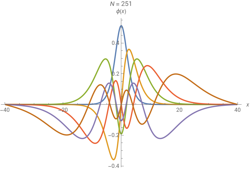
The wave functions are plotted to check if the chosen range for the position variable allows to reach the asymptotic tails.
Eigenvalues of the bounding potentials, Coulomb and harmonic oscillator, are also computed.
(*Hamiltonian*)(*H=T(p)+V(x)with[x,p]=ihbarand-∞<x<+∞*)(*ComputationofthesolutionsofHϕ(x)=Eϕ(x)*)(*System*)Tp[p_]:=d=2;(*dimensionlessparameterD*)Vx[x_]:=-+(*Listofquantumnumbers:n=0,1,...*)listn={0,1,2,3,4,5};llistn=Length[listn];le1=Table[{0,0},{i,1,llistn}];le2=Table[{0,},{i,1,llistn}];le3=Table[{0,0},{i,1,llistn}];le4=Table[{0,0},{i,1,llistn}];(*OddnumberNofmeshpoints(nMP)*)nMP=251;(*AccuracyincreaseswithN*)If[EvenQ[nMP],nMP=nMP+1](*Range:x∈{,}*)(*=2-ifV(x)symmetricalwithrespectto*)xinf=-40.;(*Accuracyincreaseswiththesizeoftheinterval{,}*)xsup=-xinf;(*Intermediatecomputations*)n=;h=xsup-xinf;dx=;(*ComputationoftheHamiltonianmatrixH*)t1=TimeUsed[];Hij=Table[0,{i,1,nMP-1},{j,1,nMP-1}];DoDoHij[[i,j]]=Sum2Cos(i-j)Tps,{s,1,n}+Tp[0];Hij[[j,i]]=Hij[[i,j]],{j,1,i},{i,1,nMP-1};Hij=Hij+DiagonalMatrix[Table[Vx[xinf+idx],{i,1,nMP-1}]];t2=TimeUsed[];(*DiagonalizationoftheHamiltonianmatrix*)all=Eigensystem[Hij];evalFG=Sort[all[[1]]];pos=Ordering[all[[1]]];evecFG=Table[all[[2,pos[[i]]]],{i,1,nMP-1}];t3=TimeUsed[];(*Printings*)Print["Computation of H: ",t2-t1," s"]Print["Diagonalization of H: ",Chop[t3-t2]," s"]Don0=listn[[i]];e1=Extract[evalFG[[n0+1;;n0+1]],{1}];(*EigenvaluesfromFGHmethod:*)Print["(n=",n0,") = ",e1];IfOddQ[n0],e2=N-;If[OddQ[n0],Print["(n=",n0,") = ",e2]];(*EigenvaluesforCoulombpotential:*)e3=Nn0+-;Print["(n=",n0,") = ",e3];(*EigenvaluesforHarmonicoscillator:*)le1[[n0+1,2]]=e1;If[OddQ[n0],le2[[n0+1,2]]=e2];le3[[n0+1,2]]=e3;le1[[n0+1,1]]=n0;le2[[n0+1,1]]=n0;le3[[n0+1,1]]=n0;,{i,1,llistn}ListPlotTableTablexinf+,,{i,1,nMP-1},{j,1,llistn},PlotRangeFull,JoinedTrue,InterpolationOrder2,PlotStyleThick,AxesLabel{x,ϕ[x]},PlotLabel"N = "<>ToString[nMP],PlotLegends->{Table["n = "<>ToString[listn[[i]]],{i,1,llistn}]}
2
p
2
1
2
x
2
d
x
inf
x
sup
x
sup
x
mid
x
inf
x
mid
x
inf
x
sup
nMP-1
2
h
nMP
1
nMP
2πs
nMP
2π
h
E
FGH
E
FGH
2
2
(n0+1)
E
Coul
E
Coul
1
2
1
3/2
d
1
d
E
HO
E
Coul
ih
nMP
evecFG[[listn[[j]]+1]][[i]]
dx
Computation of H: 49.438 s
Diagonalization of H: 0 s
E
FGH
E
HO
E
FGH
E
Coul
E
HO
E
FGH
E
HO
E
FGH
E
Coul
E
HO
E
FGH
E
HO
E
FGH
E
Coul
E
HO
Out[]=


Numerical solutions of equation (5) to give the envelope theory (ET) approximations.
Assembling the results from the two previous calculation to form the graph 2.
Figure 3
Figure 3
Figure 4
Figure 4
Ground (black) and first excited (gray) states of H for three values of D: accurate wavefunctions computed with the FGH method (dashed), and approximate wavefunctions computed with the ET (solid). All quantities are dimensionless.
Choice of D of the soft-Coulomb potential for the computations.
Computation of n = 0 eigenstate with the FGH method (see comments for figure 3). It may be necessary to change the global sign in order to compare with the ET solution.
Computation of n = 1 eigenstate with the FGH method (see comments for figure 3). It may be necessary to change the global sign in order to compare with the ET solution.
Computation of n = 0 eigenstate with the envelope theory.
Computation of n = 1 eigenstate with the envelope theory.
Run the following code to create the graphs once the computations for D = 0.5 are done.
Run the following code to create the graphs once the computations for D = 1 are done.
Run the following code to create the graphs once the computations for D = 2 are done.
Assembling the 3 graphs.
Figure 5
Figure 5
Dimensionless energies of the ground (3 curves below) and first excited (3 curves above) states of H as a function of D: accurate values obtained with the FGH method (solid black), upper bounds from the variational method in [9] (dashed gray), upper bounds from the ET (solid gray).
Computation of the dimensionless upper bounds for the ground state and the first excited state of the soft-Coulomb potential. See:
F. Grasselli, Variational approach to the soft-Coulomb potential in low-dimensional quantum systems, Am. J. Phys. 85 (2017) 834. [reference 9 of our paper]
https://aapt.scitation.org/doi/10.1119/1.4994809
For practical reasons, formulas below contain a supplementary factor 1/2 with respect to formulas in reference [9]. See section 3.4 in our paper.
The eigenvalues with the FGH method and the ET can be obtained with the codes given above in the section about figure 2.
CITE THIS NOTEBOOK
CITE THIS NOTEBOOK
The envelope theory as a pedagogical tool
by Claude Semay and Maud Balcaen
Wolfram Community, STAFF PICKS, June 3, 2024
https://community.wolfram.com/groups/-/m/t/3186895
by Claude Semay and Maud Balcaen
Wolfram Community, STAFF PICKS, June 3, 2024
https://community.wolfram.com/groups/-/m/t/3186895